ReGIR - An advanced implementation for many-lights offline rendering
The many-lights sampling problem
To render a 3D scene, a naive “brute-force” path tracer sends out rays from the camera, bounces the rays around the scene multiple times and hopes fingers crossed that the ray is eventually going to hit a light. In the event that the ray leaves the scene without having hit a light, the pixel stays black and you’ve done the work for nothing. On top of that if the lights of your scene are very small or very far away (or more generally, are small in solid angle at your shading point), then naively bouncing rays around is going to have a very low probability to actually hit a light source.
The solution to that in practice, rather than hoping that the rays are going to hit a light, is to purposefully choose a light from all the lights that exist in your scene, shoot a shadow ray towards that light to see if it is occluded, and if it’s not, use that light to shade the current vertex along your path. This method is called next-event estimation (NEE).
However, it isn’t that simple. The subtle question is: how do I choose the light that I shoot a shadow ray to? Do we just choose the light completely at random? That works, but from an efficiency standpoint, this is far from ideal, especially when there are tons of lights in the scene:
- I want to choose a light for my point \(X\) on a surface
- There are 1000 lights in the scene
- Only 1 light meaningfully illuminates my point \(X\), all the other 999 lights are too far away and don’t contribute much at all to \(X\)
If I choose the lights for NEE completely at random, there’s a 1/1000 chance that I’m going to choose the good light for the point \(X\). That’s not amazing and this is going to cause very high variance (i.e. very high levels of noise) in our image and our render is going to take a while to converge to a clean image.

Bottom: reference, converged image.
This scene contains ~137k emissive triangles.
Surely this is going to take a while to converge.
Note:
Unless stated otherwise, all images in this blog post are rendered with 0 bounces (shoot a camera ray, find the first hit, do next-event estimation and you’re done). This is to focus on the variance of our NEE estimator. Adding more bounces would introduce the variance of path sampling and it would be harder to evaluate whether we’re going in the right direction or not with regards to reducing the variance of our NEE estimator.
Brief detour to the mathematics of why we have so much noise when choosing lights uniformly at random.
Ultimately, when estimating direct lighting using next-event estimation, we’re trying to solve the following integral at each point \(P\) in our scene:
\begin{equation} L_o(P, \omega_o) = \int_{A}^{}\rho(P, \omega_o, \omega_i)L_e(x)V(P\leftrightarrow x)\cos(\theta)\frac{\cos(\theta_L)}{d^2}dA_x \label{directLightingIntegral} \end{equation}
With:
- \(L_o(P, \omega_o)\) the reflected radiance of point \(P\) in direction \(\omega_o\), the outgoing light direction (direction towards the camera for example)
- \(\int_{A}\) is the integral over the surface of our lights in the scene: to estimate the radiance that our point \(P\) receives from the lights of the scene, we need a way of taking into account all the lights of the scene. One way of doing that is to take all the lights and then consider all the points on the surface of these lights. “Considering all the points of the surfaces of all the lights” is what we’re doing here when integrating over \(A\). \(A\) can then be thought of as the union of the area of all the lights and we’re taking a point \(dA_x\) on this union of areas.
- \(\rho(P, \omega_o, \omega_i)\) is the BSDF used to evaluate the reflected radiance at point \(P\) in direction \(\omega_o\) of the ingoing light direction \(\omega_i\) (which is \(x - P\)).
- \(L_e(x)\) is the emission intensity of the point \(x\)
- \(V(P\leftrightarrow x)\) is the visibility term that evaluates whether our point \(P\) can see the point \(x\) on the surface of a light or not (is it occluded by some geometry in the scene).
- \(\cos(\theta)\) is the attenuation term
- \(\cos(\theta_L)/d^2\) is the geometry term with \(d\) the distance to the point on the light
- \(x\) is a point on the surface of a light source
For brevity, we’ll use
\begin{equation} L_o(P, \omega_o) = \int_{A}^{} f(x)dx \label{directLightingIntegralBrevity} \end{equation}
with
\begin{equation} f(x) = \rho(P, \omega_o, \omega_i)L_e(x)V(P\leftrightarrow x)\cos(\theta)\frac{\cos(\theta_L)}{d^2} \label{directLightingIntegralBrevityFx} \end{equation}
In a path tracer, we usually compute the value of this integral with Monte Carlo integration:
- Pick a sample (a point on a light) \(x\) with some probability density function (PDF) \(p(x)\)
- Evaluate \(\frac{f(x)}{p(x)}\)
The average value of many of those samples will get closer and closer to the true value of equation (\ref{directLightingIntegral}) which is the value that we want to compute.
Ideally, our PDF \(p(x)\) is proportional to f(x): \(p(x) = c * f(x)\). If this is the case, then every value \(\frac{f(x)}{p(x)}\) that we compute is going to be the constant \(c\):
\begin{equation} \frac{f(x)}{p(x)} = \frac{f(x)}{c * f(x)} = \frac{1}{c} \label{ZeroVarianceEq} \end{equation}
In other words, no matter what random sample \(x\) we evaluate, we will always get the same constant value \(\frac{1}{c}\) out. This means that our estimator is going to have 0 variance. And with a zero-variance estimator we get no noise in the image (the noise that we see is just a consequence of neighboring pixels having quite a different value because of variance, even though nearby pixels on the image should probably be almost the exact same color) and the whole image converges with a single sample per pixel. Very yummy.
So the ultimate goal is to be able to sample points on lights with a distribution \(p(x)\) that follows \(f(x)\) (Eq. \ref{directLightingIntegralBrevityFx}). This means, in order of the terms of \(f(x)\):
- \(\rho(P, \omega_o, \omega_i)\): we want our sample \(x\) to follow the shape of the BSDF: don’t sample a point on a light that results in a \(\omega_i\) that is outside of the delta peak of a specular BSDF for example
- \(L_e(x)\): sample lights proportionally to their power, the more powerful the more chance the light should have to be sampled
- \(V(P\leftrightarrow x)\): sample only visible points; don’t sample a point on a light that is occluded from the point of view of \(P\)
- \(\cos(\theta)\): sample light directions while accounting for the cosine-weighted falloff at the shading point \(P\); directions closer to the surface normal contribute more than grazing ones
- \(\frac{\cos(\theta_L)}{d^2}\): favor light samples that are both closer to \(P\) (stronger due to distance attenuation) and oriented toward \(P\) (the light’s surface normal aligned with direction \(\omega_i\))
Which of those terms do we take into account when choosing a light completely at random for NEE? None of those. Hence why it’s so bad.
A much better technique already is to sample lights according to their power: before rendering starts, compute the power of all the lights of the scene and build a CDF, an alias table (or anything that allows sampling a CDF) on that list of light power. Lights can then be sampled exactly proportional to their power, meaning that we’ve gained the second term, \(L_e(x)\).
The results are already much better than uniform sampling:

Center: power proportional sampling
Bottom: reference, converged image
This scene contains ~137k emissive triangles.
This is still far from perfect obviously. 3 areas are of particular interest:

The first one is above (and below) the lamp as shown in the screenshot above. Looking at the reference image, the lamp inside the lampshade should clearly illuminate the wall behind it, above and below the lampshade but we have almost nothing here. The reason for that is the same as for the chimney below: lights are not sampled based on their distance (\(1/d^2\) in term 5. \(\frac{\cos(\theta_L)}{d^2}\)) to the shading point. Relative to the whole scene, the lights inside the lampshade and inside the chimney are not really powerful. The consequence of that is that our power-proportional sampling does not favor those lights very much (because other lights are more powerful) even though those are the lights contributing the most to the shading points above and below the lampshade and inside the chimney respectively. Those are the lights that our sampling strategy should have sampled here.

For the case of the chimney, the lack of information about visibility (term 3.\(V(P\leftrightarrow x)\)) is also an issue. Power sampling alone would not be too bad of an idea if the large light panels in the front and the back of the room were visible from inside the chimney, but that’s not the case. Those large light panels are sampled often even though they are occluded from the inside of the chimney: our sampling distribution is far from proportional to our actual integrand \(f(x)\) and we suffer from lots of noise because of that (we only have term 2. \(L_e(x)\) after all).

Bottom: Another point of view of the scene. The large quad light in the back is the only one that is able to light to back of the couch.
The case of the back of the couch is also interesting. Looking at the different point of view of the scene, we can see that the only light that is illuminating the back of the couch is the large light panel in the back of the room. All the other lights of the scene are behind the back of the couch (they are in the back of the back of the couch…. ** visible confusion **). This is a case where sampling according to term 4. \(\cos(\theta)\) would help immensely because that term here would be negative for all lights except the large light panel that matters to us.
The BSDF term 1. \(\rho(P, \omega_o, \omega_i)\) will be tackled later. For the ones screaming “light hierarchies” in the back, we’ll have a look at those later too.
Resampled Importance Sampling (RIS)
Let’s now introduce Resampled Importance Sampling (RIS).
RIS(Talbot et al., 2005) is at the heart of ReGIR. At its core, it is a technique that takes multiple samples \((X_1, ..., X_M)\) produced according to a source distribution \(p\) and “resamples” them into one single sample \(Y\) that follows a distribution \(\overline{p}\) proportional to a given (user-defined) target function \(\hat{p}\). Said otherwise, RIS takes a bunch of samples \((X_1, ..., X_M)\) (which can be produced by our simple uniform sampling or power sampling routine from before for example) and outputs one new sample \(Y\) that is distributed closer to whatever function \(\hat{p}\) we want (to be precise the sample \(Y\) will follow \(\overline{p}\) closer, not \(\hat{p}\) which may not be normalized and thus may not be a PDF).
Let’s quickly dive into a concrete example applied to our many-light sampling problem before this gets all too theoretical:
Recall that the integral that we want to solve at each point \(P\) in our scene is:
\begin{equation} L_o(P, \omega_o) = \int_{A}^{}\rho(P, \omega_o, \omega_i)L_e(x)V(P\leftrightarrow x)\cos(\theta)\frac{\cos(\theta_L)}{d^2}dA_x \label{directLightingIntegralRIS} \end{equation}
Now again, what a naive path tracer does to solve this integral is: at each point \(P\) in the scene, choose a light \(l\) randomly (uniformly, proportional to power, light hierarchies for the ones in the back, …), choose a point \(x\) on the surface of this light and evaluate equation (\ref{directLightingIntegralRIS}).
With the lights chosen uniformly, the probability of choosing the light \(l\) is \(\frac{1}{\mid Lights \mid}\) and the probability of uniformly choosing the point \(x\) on the surface of that light \(l\) is \(\frac{1}{Area(l)}\) with \(\mid Lights \mid\) the number of lights in the scene.
Our source distribution \(p\) is then defined as:
\begin{equation} p(x) = \frac{1}{|Lights| * Area(l)} \label{sourceDistributionP} \end{equation}
That explains the first part of the sentence about RIS: “it is a technique that takes multiple samples \((X_1, ..., X_M)\) produced according to a source distribution \(p\)”. We’ve got our source distribution \(p\) and we can generate samples (points on light sources) with it.
The next step is then to use RIS to “resample them into one sample that follows a distribution \(\overline{p}\) proportional to a given (user-defined) target function \(\hat{p}\).”
So first of all, what’s going to be our user-defined target function \(\hat{p}\)? Why not choose equation (\ref{directLightingIntegralRIS}) to be our target function so that RIS outputs samples that are proportional exactly to the function that we’re trying to integrate (which is ultimately the goal)? We can totally do that:

Delectable.
This runs at 0.5FPS.
Not so delectable anymore.
In effect, doing this will not be efficient, mostly because of the visibility term that requires tracing a ray, which is an expensive operation. In practice, the target function \(\hat{p}\) needs to be cheap-ish to evaluate or RIS will turn out to be computationally inefficient. This worked okay for this scene because it’s not too expensive to trace. And because power-proportional sampling does not do a catastrophically bad job at sampling the scene to begin with. The same 4000-samples-RIS NEE strategy but using uniform sampling this time isn’t as shiny:

This shows the importance of the "base sampling strategy" that the samples we feed RIS are produced with. If our **source distribution p** is very bad, RIS will have a hard time getting a good sample out of it.
So if the full equation (\ref{directLightingIntegralRIS}) is too expensive because of the visibility term, let’s define our target function \(\hat{p}\) without that visibility term:
\begin{equation} \hat{p}(x) = \rho(P, \omega_o, \omega_i)L_e(x)\cos(\theta)\frac{\cos(\theta_L)}{d^2} \label{targetFunctionPHatNoVis} \end{equation}
This is what such a target function can give us:
There are a couple of interesting things happening here with that \(\hat{p}\) from equation (\ref{targetFunctionPHatNoVis}):
- The 40000-samples RIS render doesn’t look that much better than the 1000 one
- The 40000-samples RIS render looks worse in some places than the 10 samples RIS render (mostly around the lampshade)
For 1., the likely explanation is that at M=1000 samples, the sample \(Y\) output by RIS is already distributed pretty much perfectly (almost perfectly. Looking closer at the back of the couch you see that this is still a bit noisy. The noise here comes from term 5. \(\frac{\cos(\theta_L)}{d^2}\) of equation (\ref{directLightingIntegralBrevityFx})) according to \(\hat{p}(x) = \rho(P, \omega_o, \omega_i)L_e(x)\cos(\theta)\frac{\cos(\theta_L)}{d^2}\). Adding more samples won’t make a difference since the sample is already perfect. It’s a perfect sample but only with regards to that \(\hat{p}\) without the visibility term \(V\). Because we omitted that visibility term, the distribution according to which our samples \(Y\) are produced is still not completely proportional to our ultimate goal, equation (\ref{directLightingIntegralBrevityFx}):
\begin{equation} f(x) = \rho(P, \omega_o, \omega_i)L_e(x)V(P\leftrightarrow x)\cos(\theta)\frac{\cos(\theta_L)}{d^2} \label{directLightingIntegralBrevityFxAgain} \end{equation}
That lack of proportionality to the visibility is the cause for all the rest of the noise visible in the image. Who would have guessed that visibility was important…
For 2., looking closer at the area around the green point on the left of the image, it’s noticeable that RIS with 10 candidates (M = 10) looks a bit better than M = 40000:

Bottom: M = 40000
This is because at M = 40000, our sample \(Y\) is distributed much closer to \(\overline{p}\) (remember that \(\hat{p}(x)\) isn’t necessarily a PDF, it’s not necessarily normalized. So strictly speaking, the samples \(Y\) are distributed closer to the normalized version of \(\hat{p}(x)\), which is \(\overline{p}\)) than with M = 10. However, this does not play in our favor here because of the missing visibility term. In this exact instance, getting closer to \(\hat{p}\) without the visibility term \(V\) (equation (\ref{targetFunctionPHatNoVis})) gets us further away from our goal, equation (\ref{directLightingIntegralBrevityFxAgain}):

The X axis represents all possible light samples in the scene.
The Y axis is the probability that a given distribution produces that light sample
These curves are approximate, they are just to illustrate the idea.
The curves above show us that increasing M gets us closer to \(\overline{\hat{p}}\) but in some places, this also moves us further away from the true goal which is distributing our samples \(Y\) proportional to \(f(x)\), as we can see with the dip in \(pf(x)\) on the right of the graph. That dip is caused by the light in the lampshade being occluded from the point of view of the green point. RIS will keep choosing that light because it’s close to our green point but it is occluded so most samples will end up having 0 contribution in the end and this is the cause for the variance here.
Now to get back to our numerical example of how to actually use RIS, what do we do with our target function \(\hat{p}\)? We’re going to use it to “resample” our samples \((X_1, ..., X_M)\) produced from \(p\).
Here’s the pseudocode of the RIS algorithm:

Algorithm starts at line 10. The idea is simple.
- (Line 10-11) Generate our \(M\) candidates according to the distribution \(p\) we talked about earlier. This corresponds to picking points on the surface of the lights of our scene.
- (Line 12) Compute the “resampling weight” \(w_i\) of this candidate \(X_i\).
- \(m_i\) is a MIS weight. For now, we’ll use \(m_i=\frac{1}{M}\)
- \(\hat{p}(X_i)\) is the value of the target function for the generated sample \(X_i\)
- \(W_{X_i}\) is what’s called the “unbiased contribution weight” of the sample/candidate. This term will be thoroughly detailed in the next sections. For now, we’ll use \(W_{X_i}=\frac{1}{p(X_i)}\), the inverse of the probability of picking that point \(X_i\) on that light in the scene the point belongs to.
- (Line 14) With these weights \(w_i\), we are now going to choose a sample \(X_i\) proportionally to its weight \(w_i\):
- Let’s say we have \(M=3\) candidates. We compute their resampling weights \(w_i\) and obtain \((w_1, w_2, w_3)=(1.2, 2.5, 0.5)\). The randomIndex() function can then be used to obtain the sample \(X_i\). Concretely in this example, the probability of choosing \(X_1\), \(X_2\) or \(X_3\) with the random index \(s\) is then:
With the random index \(s\) chosen, we can retrieve the final sample \(Y\): the output of RIS. This the sample \(Y\) that we can evaluate NEE with.
Now, in Monte Carlo integration, we need the probability (PDF) of sampling a given sample. This also applies to next event estimation as you may know: when you sample a light in the scene, you divide by the probability of sampling that light when evaluating the radiance contribution of that light at the point you’re shading.
RIS is no exception to that. RIS returns one light sample \(Y\) and its weight \(W_Y\) from the \(M\) light samples that we fed it. If we want to use that light sample \(Y\) for evaluating NEE, we’re going to need its PDF. The hard truth is that RIS “mixes \(M\) samples together” and as a result, we can’t (Bitterli et al., 2020) easily compute the PDF of the resulting sample \(Y\). What we can compute however, is an estimate of its PDF. That’s what the \(W_Y\) computed at line 17 of the algorithm is. This estimate converges to the inverse PDF \(\frac{1}{\overline{p}(Y)}\) of \(Y\) as the number of candidates \(M\) resampled increases. If we then want to divide by the PDF of our sample \(Y\), we can instead multiply by that estimate of the inverse PDF \(W_Y\) and achieve the same result.
As a matter of fact, a sample output by RIS can be used for evaluation as simply as:
\begin{equation} f(Y)W_Y \end{equation}
that is: evaluate the function you want to integrate with the sample \(Y\) and multiply by \(W_Y\) (the estimate of its inverse PDF \(\frac{1}{\overline{p}(Y)}\)) instead of dividing by \(p(x)\) as we would do with non-RIS sampling schemes.
For our direct lighting evaluation case, we can use \(Y\) as:
\begin{equation} L_o(P, \omega_o) = f(P, \omega_o, \omega_i)V(P\leftrightarrow Y)\cos(\theta)\frac{\cos(\theta_L)}{d^2}W_Y \end{equation}
with \(\omega_i\) the direction towards the light sample (point on the surface of a light) \(Y\) from \(P\).
So to recap:
- RIS takes \(M\) samples as input
- Those \(M\) samples are distributed according to a given distribution \(p\) that is easy to sample from (power sampling in the screenshots above)
- Evaluate the weights \(w_i\) for all these samples
- Choose one sample \(Y\) from \((X_1, ..., X_M)\) proportional to its weight
- Compute \(W_Y\) for that sample \(Y\)
- Evaluate NEE with that sample \(Y\)
And this is done at every shading point in the scene.
ReGIR : Reservoir-based Grid Importance Resampling
The algorithm
ReGIR is a light sampling technique built on top of RIS that was first described in the paper by Boksansky et al., 2021 (Boksansky et al., 2021). Boissé, 2021 (Boissé, 2021) also proposed something similar but based on a hash grid. The idea is to have a grid (let’s assume a regular grid for now) built over your scene, and then, in a prepass to the rendering process:
- For each cell of the grid, consider the point at the center of the grid
- Sample a few lights, \(L = 32\) (\(L\) for lights) for example, using a simple sampling technique (power sampling for example)
- Resample those \(L\) lights with RIS by estimating the contribution of each of those \(L\) samples to the point at the center of the grid cell
- This outputs one light sample that is stored in the grid cell
- Repeat the process a certain number of times, \(R = 64\) (\(R\) for reservoirs) to get more light samples (reservoirs) in each grid cell
- At path tracing time, when evaluating NEE, find out which grid cell your shading point falls into
- Get a few lights from that grid cell, \(S = 4\) (\(S\) for shading) for example.
- Resample those \(S\) light samples again with RIS
- This outputs one final light sample
- Shade that light sample for NEE
Essentially what this accomplishes is that it precomputes a bunch of light samples for each grid cell ahead of time, and then we can use these precomputed light samples at shading time for NEE, instead of our regular sampling technique.
The good bit here is the target function that we can use in step 2. If we call \(P\) the center of our cell, we can use:
\begin{equation} \hat{p}(x) = \frac{L_e(x)}{|P - x|^2} \label{regirGridFillTargetFunction} \end{equation}
that is, a target function that not only contains the power of the light but also the distance to the light. The result is that our grid cells are going to contain \(R\) light samples (or reservoirs as we’re using reservoirs to store the output of RIS here, as proposed in the ReGIR paper) that take power and distance into account. These power-distance light samples are then used at path tracing time for NEE (by looking up in which grid cell our shading point is) and completely replace the simpler power-proportional samples that we’ve been using until now. So now our light sampling technique can take distance into account to produce its samples. Let’s see how much of a quality difference that makes:
Quick notes: For now, NEE is performed with a single light sample per shading point \(S = 1\), as opposed to using RIS as in the introduction to RIS or using \(S = 4\) as in step 7. ATS is an implementation of (Conty Estevez & Kulla, 2018) and SAH/SAOH are the cost functions used when building the tree. The SAOH is supposedly of higher quality but it performs very poorly in the white room scene (a behavior that I could verify in Blender and Falcor) so that’s why the SAH is going to be used in that scene instead of the SAOH, just to get the maximum quality out of the tree. In every other scene however, the SAOH is a noticeable improvement. This may be because of all the tiny triangles (some are even degenerate and have 0 area) that the white room contains. If I ever find the bad SAOH results in the white room to be due to a bug, I’ll update this blog post. Unless stated otherwise, all ATS renders are done with a binned builder, 64 bins, built over all the emissive triangles of the scene, as low as 1 emissive triangle per leaf of the tree, no adaptive splitting.
Commenting on the white room results first, the behavior is a bit similar to what we had with RIS and the 40000 samples, except it’s worse. The lampshade at the ceiling is almost completely black past \(L = 16\)! And that’s not buggy, the image will converge correctly eventually, that’s just very bad variance. That’s because the light samples that we use for NEE are now distributed according to the simple target function of equation (\ref{regirGridFillTargetFunction}), which misses almost all the terms of our ultimate goal, equation (\ref{directLightingIntegralBrevityFx}). Compared to simple power sampling, we gained the distance term \(\frac{1}{d^2}\) but not the other terms and we get into a similar situation as before (in the introduction to RIS section where we used \(\hat{p}\) without the visibility term) where, in some places of the scene, RIS actually moves us further away from the ideal distribution. That’s the case for the exterior of the lampshade where most samples end up sampling the light inside the lampshade but that light is actually behind the surface normal and occluded: all bad samples. But getting access to spatial sampling did help in the chimney area and above and below the blue lampshade on the right of the image.
In the Bistro, things look quite a bit better for ReGIR and increasing \(L\) results in better and better samples for NEE. That Bistro scene suffers less from that issue of “RIS moving us away from the ideal target distribution” and ReGIR now significantly outperforms power sampling at equal sample count (just 1SPP in the above screenshots). We’ll have equal-time comparisons later.
Yet, those renders are still far from perfect, especially in the white room. So can we do better?
A better grid
Let’s start by addressing the elephant in the room: the regular grid.
Bad. Mostly because there is a ton of empty space in a regular grid: grid cells that contain no scene geometry at all and that our NEE is never going to query because no ray will ever hit geometry in those grid cells. This has us filling the grid (computational time) and storing reservoirs in those grid cells (VRAM usage) for nothing. And a lot of them.
The better data structure that I ended up using for ReGIR is a hash grid, inspired by the spatial hashing of Binder et al. 2019 (Binder et al., 2019). This works by first hashing a “descriptor”, getting a hash key out of that hash operation, and using that hash key to index a buffer in memory: that index in the buffer is where we can store information about the grid cell: the reservoirs of our cells and more.
Probably the most simple and useful descriptor that can be used to start with is just the 3D position in the scene:
unsigned int custom_regir_hash(float3 world_position, float cell_size, unsigned int total_number_of_cells, unsigned int& out_checksum) const
{
	// The division by the cell_size gives us control over the precision of the grid. Without that, each grid cell would be size 1^3
	// in world-space
	unsigned int grid_coord_x = static_cast<int>(floorf(world_position.x / cell_size));
	unsigned int grid_coord_y = static_cast<int>(floorf(world_position.y / cell_size));
	unsigned int grid_coord_z = static_cast<int>(floorf(world_position.z / cell_size));

	// Using the two hash functions as proposed in [WORLD-SPACE SPATIOTEMPORAL RESERVOIR REUSE FOR RAY-TRACED GLOBAL ILLUMINATION, Boisse, 2021]
	unsigned int checksum = h2_xxhash32(grid_coord_z + h2_xxhash32(grid_coord_y + h2_xxhash32(grid_coord_x)));
	unsigned int cell_hash = h1_pcg(grid_coord_z + h1_pcg(grid_coord_y + h1_pcg(grid_coord_x))) % total_number_of_cells;

	out_checksum = checksum;
	return cell_hash;
}
The hash function computes both a hash-key ‘cell_hash’ that will be used to index the hash grid buffer and a checksum that can be used to detect collisions: it can happen that two very different positions in world space end up yielding the same ‘cell_hash’, but chances are that the ‘checksum’ is going to be different, allowing us to detect the collision. If it happens that the checksum is also the same, that’s very unfortunate and we’ll end up using the reservoirs of one grid cell to shade another cell in the grid. This is not the end of the world but that’s going to increase variance when that happens. ‘checksum’ uses a full 32-bit unsigned integer however so this situation should happen extremely infrequently. ‘cell_hash’ on the other hand is computed modulo ‘total_number_of_cells’. This is such that we do not get an index out of the hash function that does not fit in our hash grid buffer (‘total_number_of_cells’ is the size of our hash grid buffer, allocated to a fixed size in advance).
Resolving collisions is done with linear probing as presented by Binder et al. in their talk (Binder et al., 2019)., it’s very simple although be a bit more effective. My tests suggest that the hash table starts to struggle a bit with collisions at ~85% load factor (load factor is the proportion of cells occupied in the table). Considering that my tests were done with a maximum of 32 steps for linear probing, that’s not amazing when compared to the results of the survey on GPU hash tables from Awad et al. 2022 (Awad et al., 2022). Their introduction reports a probe count of only 1.43 at load factor 99% for a BCHT (bucketed cuckoo hash table) scheme, but linear probing is already struggling at load factor 95% with a probe count of 32…
The consequence of a probing scheme that struggles is that we need to maintain a relatively low load factor to avoid suffering from unresolved collisions and lower performance because of longer probe sequences. This means more wasted VRAM as the hash grid buffer must be larger than necessary to achieve a low enough load factor. My implementation resizes the buffer of the hash grid (and reinserts the grid cells of the old hash table in the new hash table) automatically if the load factor exceeds 60% and I’ve found this enough of a “target load factor” in practice.
The above screenshots show that the number of collisions left unresolved increases as the load factor increases. Unresolved collisions manifest as black cells in the debug view. When doing NEE, this means that we will not be able to access the hash grid data at all for that cell. That cell will thus be completely black as NEE will not have any light sample to work with. The solution that I’ve found to that is just to fallback to a default light sampling strategy if that happens. This will have higher variance than ReGIR obviously (that’s the goal after all, we want ReGIR to be better than just a simple light sampling strategy) but at least it will not be conspicuously biased.
One that question that I personally have at this point: what’s the impact of the hash grid resolution on quality and rendering efficiency? Well, let’s have a look. A visualization of the grid sizes used for this comparison is given below:
And a table to sum up the number of samples needed for convergence to a given quality target (given below) as well as the time it took to render that many samples:
| Time to converge | Power sampling only | Light tree ATS | ||||||
|---|---|---|---|---|---|---|---|---|
| Grid size: | 8 | 2 | 1 | 0.5 | 0.25 | 0.125 | ||
| The white room (75%) | 10.13s | 13.86s | 14.53s | 15.32s | 15.93s | 19.08s | 8.6s | 10.47s |
| Bistro (25%) | 6.7s | 5.44s | 5.41s | 5.77s | 7.12s | 11.37s | 48.23s | 6.65s |
| Samples to converge | ||||||||
| Grid size: | 8 | 2 | 1 | 0.5 | 0.25 | 0.125 | ||
| The white room (75%) | 3257 | 4395 | 4565 | 4691 | 4712 | 4717 | 3166 | 4876 |
| Bistro (25%) | 1519 | 1214 | 1180 | 1171 | 1164 | 1162 | 13041 | 1794 |
At this point of the implementation, the grid size affects quality for the worse in the white room, noticeably, most likely because of the very imperfect target function that we’re using and the white room scene seems very sensitive to it. On the Bistro however, we do see an increase in quality (lower sample count to converge) until we hit diminishing returns in between grid size 1 and grid size 0.5. The increase in quality is directly visible in some areas of the Bistro where spatiality matters (and thus a higher grid resolution matters):

Right: grid size 8
Both 32SPP. L=32, R=64, S=1.
Reminder: \(L\) is the number of light samples per reservoir of each grid cell. \(R\) is the number of reservoirs per each grid cell. \(S\) is how many reservoirs we resample per shading point at NEE time.
In terms of methodology for measuring what’s reported in the table above, the scenes are rendered and frames accumulated until a certain proportion of the pixels of the image have reached a given estimated variance threshold. For both scenes above, the variance threshold used was 0.075. Rendering stopped after 75% of pixels have reached that threshold variance in the white room and 25% for the Bistro (indicated in the brackets).
In the end, this hash grid saves us a ton of VRAM but also, very importantly, allows us to have geometric information about the cells of the grid: because we allocate cells in the buffer when a ray hits the scene (we hash the position and insert in the right place if that grid cell hasn’t been inserted in the hash grid before), we only ever store grid cells on the actual geometry of the scene and we know what that geometry is like since we used that geometric information to compute the hash in the first place. That geometric information attached to the grid cells is something that will come in very handy for improving the quality of ReGIR samples.
Improving the target function
So far, the target function that we’ve been using to resample our light samples \(L\) into reservoirs \(R\) during grid fill has been:
\begin{equation} \hat{p}(x) = \frac{L_e(x)}{|P - x|^2} \label{regirGridFillTargetFunctionAgain} \end{equation}
We would like this target function to get as close as possible to the full \(f(x)\) ideal target function. With the regular grid, we had to estimate the contribution of the \(L\) lights sampled to the center of the grid cell because we couldn’t really do better. With the hash grid now, we have access to way more information about the grid cell. For the ray that inserted that grid cell in the hash grid, we have:
- A point on the surface of the scene in that grid cell \(P_c\) (for Point_cell)
- The surface normal at that point \(N_c\) (for Normal_cell)
- The material at that point \(M_c\) (for Material_cell)
Note that if multiple rays hit the same hash grid cell and all want to insert their point/normal/material into the grid cell, only one of those rays will win the atomic insertion operation and so the grid cell will be “geometrically represented” only by one point/normal/material = only one of all those rays that hit the cell. This can cause some issues as we’ll see just below.
With these new pieces of information, let’s review which terms we’ll be able to incorporate into our grid-fill target function:
- Term 1. \(\rho(P_c, \omega_o, \omega_i)\) of \(f(x)\) can be added since we have the material of the grid cell (the material at the point in the grid cell rather). We will still omit this one for now and reserve it for a later dedicated section of this blog post.
- Term 2. \(L_e(x)\): we already had this one even with the regular grid
- Term 3. \(V(P_c\leftrightarrow x)\): we can have the visibility term by tracing a ray between the point of the grid cell and the point of the light sample (we’ll see that this is not a super good idea however)
- Term 4. \(\cos(\theta)\): we have the surface normal so this one fits too
- Term 5. \(\frac{\cos(\theta_L)}{d^2}\): we already had \(\frac{1}{d^2}\) although this was with respect to the center of the cell. We can now compute \(\frac{1}{d^2} = \frac{1}{|P_c - x|^2}\) given a point on the surface of the scene in the grid cell so that’s going to be more precise. For \(\cos(\theta_L)\), we could already have added this one even with the regular grid, by computing it also with respect to the center of the grid cell, but the original ReGIR article didn’t use it so we started without it as well. We’ll add it to our new target function now.
With that, this is our new target function, for a light sample \(x\) (point on a light):
\begin{equation} \hat{p}(x) = L_e(x)V(P_c\leftrightarrow x)\cos(\theta)\frac{\cos(\theta_L)}{|P_c - x|^2} \label{regirGridFillTargetFunctionBetter} \end{equation}
with
- \(\cos(\theta) = dot(N_c, normalize(x - P_c))\).
- \(\cos(\theta_L) = dot(normalize(P_c - x, N_L))\), where \(N_L\) is the normal at point \(x\) on the surface of the light source
Where are we now in terms of quality with that new target function?
ReGIR with \(\hat{p}(x) = L_e(x)\cos(\theta)\frac{\cos(\theta_L)}{|P_c - x|^2}\) is between 1.5x and 2x slower than power sampling, depending on the scene so power sampling 2SPP corresponds roughly to an equal-time comparison with ReGIR and that \(\hat{p}(x)\).
As expected, adding \(\cos(\theta)\) to the target function helps a lot. It’s most visible on the lampshade at the ceiling in the white room where samples targetting the light inside the lampshade (which were the samples contributing the most with \(\hat{p(x)} = \frac{L_e}{d^2}\)) are now discarded because they are below the surface. In other scenes, no such extreme case so the improvement from \(\cos(\theta)\) is more modest.
Adding \(\cos(\theta_L)\) helps even more than \(\cos(\theta)\) because my renderer does not allow back-facing lights. The result is that around half the lights of these scenes are discarded from the onset, during grid fill when the target function contains that \(\cos(\theta_L)\) term. We end up with samples that are distributed much more often on lights that are not back-facing to the shading points, that is, lights that actually have a non-zero contribution.
Adding visibility also reduces variance massively in all scenes but the white room is the one that benefits the most from it. However, the renders with visibility in the target function look a bit blocky, artifacty, not clean, not uniform, … It’s not that delectable. The major issue I think is that:
- Visibility is quite a sensitive term: it completely zeroes out the target function if the sample is occluded. However, during grid fill, we’re computing visibility between the representative point of the grid cell \(P_c\) and the point on the light \(x\). Always using \(P_c\) here is a problem because that point does not represent the grid cell very well in most situations. The visibility term for a given light may vary significantly within a grid cell so computing the visibility of the samples only, and always, from \(P_c\) isn’t great and this results in grid cell artifacts where noise increases significantly where that \(P_c\)-visibility assumption turns out to be wrong: light samples will never be selected by the grid fill even though they have a non-zero contribution at some points in the grid cell other than \(P_c\) (this is a source of bias for those wondering, and the subject is tackled in a following section).
The recap of that visibility-term precision is that we should have more precision where lighting frequency is high: if visibility changes faster than the precision of the hash grid, then that’s where we run into issues. More on that in the section on potential improvements.
But when visibility is accurate, it looks quite good: the walls on the left and right, the ceiling and the floor: flat surfaces where there is little risk of making visibility-term mistakes.
| Time to converge | Power sampling only | Light tree ATS | ||||
|---|---|---|---|---|---|---|
| Target function | Le/d^2 | +cos(theta) | +cos(theta_L) | +V | ||
| The white room (75%) | 13.48s | 11.3s | 8.46s | 5.38s | 6.252s | 10.47s |
| Bistro (50%) | 12.36s | 9.1s | 5.86s | 33.82s | 63.78s | 13.42s |
| BZD measure-seven(75%) | 9.24s | 7.68s | 5.6s | 31.9s | 46.88s | 11.26s |
| Samples to converge | ||||||
| The white room(75%) | 4690 | 3842 | 2823 | 387 | 3141 | 4865 |
| Bistro(50%) | 2319 | 1626 | 1001 | 810 | 20781 | 3273 |
| BZD measure-seven;(75%) | 2545 | 2021 | 1450 | 1391 | 17086 | 3485 |
Although visibility looks quite good in terms of variance (omitting the artifacts which we’ll address very soon), it is clearly isn’t very efficient in general. It performs well in the white room because this is a scene that has complicated visibility (despite looking like a simple scene) and that is also fairly fast to trace. In the two other scenes however, it is clearly way too expensive to be worth it in terms of rendering efficiency (but it does improve quality as we can see by the lower sample counts needed to converge to the same quality).
Before having a closer look at what we can do for visibility sampling, let’s address the artifacts.

For the case of the couch, the issue is that the point \(P_c\) and surface normal \(N_c\) (in green) used by that grid cell (the ones that were inserted at the creation of the grid cell) are only on one side of the couch. But during NEE, we may have shading points on both “sides of the couch”. This creates a situation where some shading points (in red) are using ReGIR samples that were produced with a grid cell that has geometric information (and thus grid fill target function) completely different from the geometry at that shading point. When this happens, we get bias in the form of darkening (or bad variance instead of bias if the ReGIR implementation is unbiased, as explained later).
Note on bias
In practice, when some shading points are not able to find NEE samples at path tracing time because of large differences between the grid fill target function and the surface at the shading point, we get a large amount of bias in the form of darkening. This is because some lights will never be able to be sampled from those shading points because the grid fill target function is 0 for those light samples, even though they would have had non-0 contribution if evaluated by NEE for that shading point. The reason that the screenshots above manifest large amounts of noise in those regions instead of darkening is because the implementation is unbiased and compensates for those missing samples, as explained in a later section.
And easy solution to fix this is to introduce the surface normal in the hash grid function:
unsigned int hash_quantize_normal(float3 normal, unsigned int precision)
{
    unsigned int x = static_cast<unsigned int>(normal.x * precision) << (2 * precision);
    unsigned int y = static_cast<unsigned int>(normal.y * precision) << (1 * precision);
    unsigned int z = static_cast<unsigned int>(normal.z * precision);

    return x | y | z;
}

unsigned int custom_regir_hash(float3 world_position, float cell_size, unsigned int total_number_of_cells, unsigned int& out_checksum) const
{
	// The division by the cell_size gives us control over the precision of the grid. Without that, each grid cell would be size 1^3
	// in world-space
	unsigned int grid_coord_x = static_cast<int>(floorf(world_position.x / cell_size));
	unsigned int grid_coord_y = static_cast<int>(floorf(world_position.y / cell_size));
	unsigned int grid_coord_z = static_cast<int>(floorf(world_position.z / cell_size));

	unsigned int quantized_normal = hash_quantize_normal(surface_normal, primary_hit ? ReGIR_HashGridHashSurfaceNormalResolutionPrimaryHits : ReGIR_HashGridHashSurfaceNormalResolutionSecondaryHits);

	// Using the two hash functions as proposed in [WORLD-SPACE SPATIOTEMPORAL RESERVOIR REUSE FOR RAY-TRACED GLOBAL ILLUMINATION, Boisse, 2021]
	unsigned int checksum = h2_xxhash32(quantized_normal + h2_xxhash32(grid_coord_z + h2_xxhash32(grid_coord_y + h2_xxhash32(grid_coord_x))));
	unsigned int cell_hash = h1_pcg(quantized_normal + h1_pcg(grid_coord_z + h1_pcg(grid_coord_y + h1_pcg(grid_coord_x)))) % total_number_of_cells;

	out_checksum = checksum;
	return cell_hash;
}
The case of the lampshade is a bit different and does not have to do with surface orientation but rather with lighting frequency. If the grid cells are too large, the approximation that visibility is only computed from \(P_c\) for the whole grid cell falls apart and we get grid cell artifacts. A proper solution to that would increase grid cell resolution in areas of high lighting frequency. More about that in “Limitations and potential improvements”. In the meantime, something we can do to help with that issue is to jitter the shading points: when evaluating NEE, jitter the shading point position randomly and only then look up which grid cell that jittered shading point falls into. We then use ReGIR light samples of that grid cell for NEE.

Grid cells artifacts are massively reduced and the image looks much cleaner.
Jittering the NEE shading point’s position completely randomly (i.e. with random vec3()) isn’t really a good idea for one main reason: the jittered point may end up outside of the scene. For a shading point on a wall of the white room for example, jittering in the direction normal to the wall will move the point either outside of the room (point jittered in the direction opposite to the normal of the wall) or into the empty space of the room (point jittered in the direction of the normal of the wall). In any case, this is a risk of having no grid cell (and thus light samples) to fetch at that jittered position, which is biased. One solution is to jitter the point again (and even up to a maximum of N times) if the first jittering failed (no grid cell was found at the jittered position), hoping that a second jittering will jitter correctly this time. This is however expensive as each jittered point needs to be hashed and looked up into the hash grid, with collision resolution and everything that the implementation entails. The better solution that I use is to always jitter the point in the tangent plane of the surface normal. With the example of the wall in the white room, this would jitter the point exactly in the direction of the wall and thus not miss the surface of the scene. This optimization helps a bit with performance as fewer jitter retries are necessary to find a valid jittered position.
float3 jitter_world_position_tangent_plane(float3 original_world_position, float3 surface_normal, Xorshift32Generator& rng, float grid_cell_size, float jittering_radius = 0.5f)
{
	// Getting the tangent plane vectors from the normal. The ONB can be built
	// with the method of your choice.
	float3 T, B;
	build_ONB(surface_normal, T, B);

	// Offsets X and Y in the tangent plane
	float random_offset_x = rng() * 2.0f - 1.0f;
	float random_offset_y = rng() * 2.0f - 1.0f;

	// Scaling by the grid size
	float scaling = grid_cell_size * jittering_radius;
	random_offset_x *= scaling;
	random_offset_y *= scaling;

	return original_world_position + random_offset_x * T + random_offset_y * B;
}
Both techniques can fail however and never find a good jittered point, in which case, to avoid bias (or variance if the implementation is unbiased), my implementation falls back to using the non-jittered original shading point for looking up the grid cell and fetching the light samples.
Most of the grid cell artifacts are gone but shooting visibility rays during the grid fill pass is still too expensive. If we still want to have some notion of visibility sampling (and we do), we need something cheaper.
NEE++
Next Event Estimation++, first proposed by Guo et al. in 2020 (Guo et al., 2020), is a visibility caching algorithm based on a voxel grid. The idea is that, for each shadow ray that you shoot during rendering between a shading point \(P\) and a point on a light \(P_L\), you find the two voxels that these two points belong to (assuming you have built a regular grid structure over your scene) and you accumulate whether that shadow ray was occluded for these 2 voxels (using a linear buffer to store the voxel-to-voxel visibility matrix of the scene or any suitable data structure; I use a hash grid again, to avoid storing irrelevant voxel-to-voxel pairs).
As more shadow rays, are traced, voxel pairs start accumulating visibility information in the scene in the form of a probability \(p = \frac{visibleRays}{totalRaysTraced}\). Guo et al. used that visibility probability between 2 voxels in 2 different ways for backwards path tracing:
- Shadow rays russian roulette: if there is a 99% chance that 2 voxels are occluded, then 99% of the time we may as well assume that the shadow ray is going to be occluded without even tracing it. 1% of the time we still trace the ray and weight the NEE contribution by that 1% probability, as in russian roulette. This approach of using the visibility probability increases variance but should improve rendering efficiency by not tracing obviously occluded rays.
- Build a sampling distribution for each voxel to guide the sampling of lights for NEE based on the voxel-to-voxel visibility. This approach reduces the variance of the NEE estimator by incorporating some measure of visibility in the sampling of lights.
For ReGIR, we’re going to use the visibility probability directly in the grid-fill target function, to aid in sampling visible lights (similar to step 2. in that respect):
\begin{equation} \hat{p}(x) = L_e(x)V_{NEE++}(P_c\leftrightarrow x)\cos(\theta)\frac{\cos(\theta_L)}{|P_c - x|^2} \label{regirGridFillTargetFunctionBetterNEEPusPlus} \end{equation}
with \(V_{NEE++}\) the visibility probability returned by querying the NEE++ data structure for the voxels of point \(P_c\) and \(x\). For lights that are obviously occluded (behind a wall, inside a lampshade, …), this should allow the target function to reject those lights since the visibility probability should be 0 (note that allowing a visibility probability of exactly 0 is biased in most cases and so in practice, we can clamp that probability to a minimum of 0.01 for example). If \(V_{NEE++}\) is low but not 0, then this will lower the resampling weight of that light sample during the grid fill and that maybe-occluded (or rather, partially-occluded) light will be selected less often.
Querying visibility that way amounts to a few math ops to compute the position in the grid and then a lookup into the visibility-accumulation buffer. It’s obviously way cheaper than tracing rays, but if this is only an approximation, how well does it perform in terms of quality?
| Time to converge | |||
|---|---|---|---|
| Target function | No NEE++ | NEE++ | Full visibility |
| The white room (75%) | 9.34s | 1.87s | 3.80s |
| Bistro (50%) | 7.17 | 5.79s | 37.52s |
| BZD measure-seven;(75%) | 5.95s | 5.32s | 32.07s |
| Samples to converge | |||
| The white room;(75%) | 2392 | 419 | 189 |
| Bistro;(50%) | 888 | 636 | 594 |
| BZD measure-seven;(75%) | 1149 | 878 | 762 |
The white room is again the scene that benefits the most from visibility sampling, with a dramatic 5x improvement with NEE++. The other scenes show a more modest improvement but still an improvement. NEE++ also becomes important in the target function used during shading (when \(S\) > 1), such that the visibility sampling benefits during grid fill do not vanish because of the non-visibility-aware resampling that would happen at shading time without NEE++ in that target function as well.
BSDF resampling
Of all the terms in equation (\ref{directLightingIntegralBrevityFx}), the BSDF \(\rho(P, \omega_o, \omega_i)\) is the only term that we haven’t tackled yet. Why not also add it to the grid fill target function?
\begin{equation} \hat{p}(x) = \rho(P_c, \omega_o, \omega_i)L_e(x)V_{NEE++}(P_c\leftrightarrow x)\cos(\theta)\frac{\cos(\theta_L)}{|P_c - x|^2} \label{regirGridFillTargetFunctionBetterNEEPusPlusBSDF} \end{equation}
Importantly, \(\omega_o\) here is \(camera - P_c\), which is not exactly the outgoing light direction that we’re going to need during shading. Indeed, at NEE time, the outgoing light directions at our NEE shading points \(P_s\) are going to be \(camera - P_s\), not \(camera - P_c\). The approximation gets worse the lower the roughness of the BSDF (or the more view-dependent the BSDF). At high enough roughness however, even this approximation is enough to get a slight boost in quality on glossy surfaces.
Note:
I haven’t found a solution to have the BSDF term work at secondary hits because we don’t have the view direction anymore there. At first hits, we could use the direction to the camera but the view direction at secondary hits could be anything, any direction that a ray at the first hit bounced into. I’ve actually measured multiple times that just ignoring that fact increases variance: using ReGIR light samples for secondary hits next-event-estimation that were produced during the grid fill with a BSDF term that uses the direction towards the camera as the outgoing light direction is not a good idea.
That’s why in my implementation, the first and secondary hit grid cells are decoupled, they are 2 independent hash grids, with a different number of reservoirs per cell, different target function (secondary hits don’t include the BSDF term), …
At roughness 0, the specular part of the BSDF is a delta distribution and we cannot sample that delta peak with proper BSDF sampling, so all specular highlights are missing, we need MIS for those. The improvement is slightly noticeable on the floor and on the TV in the white room at roughness 0.1, but it’s not outstanding quality either.
A little bit visible on the floor in the Bistro too:

So far, I personally don’t find the increase in quality to be that interesting. It’s something but not that succulent. So what can we do? The reason why this isn’t as good as we could have expected is mainly because of the \(P_c = P_s\) approximation (with \(P_s\) our shading points during NEE). If grid cells are too large, this approximation falls apart and the grid fill isn’t able to produce light samples that are going to be relevant on the glossy surface at all points \(P_s\) in the grid cell at NEE time. A higher resolution grid could help but this would also increase the cost of filling the grid because that’s more grid cells to fill (and memory usage is also going to increase). But what if we could increase the resolution of the grid but only on glossy surfaces, i.e. where a higher grid resolution is actually going to help.
Now a finer grid actually helps noticeably and we don’t need insets to notice the difference. Increasing the number of light samples resampled into each reservoir of the grid also helps a lot as we can see going from \(L=32\) to \(L=128\). It also helps on other areas of the scene, not just the glossy highlights (back of the couch, above the blue lampshade, …). Resampling 128 light samples for each reservoir of each grid cell is becoming a bit expensive though so it’s time to introduce something that’ll let us get way more quality for not too big of an increase in computational cost.
Note:
There are product sampling methods out there [(Heitz et al., 2016), (Heitz et al., 2018), (Hart et al., 2020), (Peters, 2021)] that aim at sampling directly the product of the BSDF and the incoming radiance (instead of relying on resampling to do that). These methods could potentially be a very good addition here (and in pretty much any light sampling implementation) but I haven’t had the chance to try those yet.
Spatial reuse
With the title of this section being “Spatial reuse”, those familiar with ReSTIR will start to recognize the pattern: initial candidates (grid fill) -> temporal reuse -> spatial reuse. The goal of the spatial reuse pass is to help a given grid cell get better light samples for itself by looking at what light samples the neighboring grid cells have produced so far. Those neighboring light samples are resampled (resampling again, it’s RIS all the way down) into a reservoir that is then stored in the grid to be used at shading time (we do not use the output of the grid fill for NEE anymore, now we use the output of the spatial reuse pass). Conceptually, it’s really not that different from the resampling that happens during grid fill where we resample a few light samples (\(L\)) into a reservoir. The difference is that here, the “light samples” are the reservoirs of the neighboring grid cells, not just pure light samples directly produced by a light sampling technique.
The whole point of spatial reuse is to amortize the cost of sampling:
- During grid fill, we’re resampling “raw light samples” into a single reservoir that is the output of the grid fill pass
- During the spatial reuse, we’re resampling those reservoirs output from the grid fill. Those reservoirs already contain the work of resampling \(L\) raw light samples. So if we resample 5 spatial neighbors, that each produced their reservoirs with \(L=32\) light samples, the reservoir that we’re going to output from the spatial reuse pass is going to contain the resampling of \(L_{spatial} = L*5 = 160\) light samples. With just 5 more resampling operations, we went from an effective “reservoir quality” of 32 light samples to 160. This is why spatial reuse makes sense, because it improves quality a lot for a lot cheaper than it should have been without spatial reuse.
Now also comes the question of “how to fetch” a neighbor to resample from. A hash grid is not a regular grid, it’s not as simple as offsetting your current point in a given direction by the size of the grid cells of your grid to get a new grid cell (a neighbor) to resample from. This could actually work like that with a hash grid but as long as the hash function is simple. We’ve already introduced the surface normal into the hash function and also the roughness of the material to get a higher grid resolution where it matters, so clearly, our grid cells are not just simple cubes anymore and it’s not easy to know where your neighbors are, let alone what descriptor (the information given to the hash function: spatial position, surface normal, roughness, …) to hash to find the index in your hash grid buffer where your neighbor information is located in memory.
Nonetheless, simply offsetting the point \(P_c\) in a random direction (actually, in the tangent plane of the surface, as already described) and hoping to find a neighbor is exactly what I did, only because I couldn’t find anything better and simple enough.
So for a given grid cell that we want to do spatial reuse from, with geometric information:
- \(P_c\) the surface point of the grid cell
- \(N_c\) the surface normal of the grid cell
- \(M_c\) the material of the grid cell at \(P_c\)
We can look in the hash grid for a neighbor to reuse from by hashing the descriptor:
- \(P_c + vec3(rng()) * reuseRadius\) (or randomly in tangent plane)
- \(N_c\).
- \(M_c\) (and using the roughness of that material to decide on grid resolution)
So essentially, we’re allowing reuse only on neighbors that have similar geometrical information as the point we’re doing the reuse at. From this angle, this does not sound so stupid anymore: we wouldn’t want to reuse from a neighbor that has a wildly different surface normal than our center grid cell because chances are that the light samples (produced by the grid fill) at that neighboring grid cell are not going to be good at our center cell if the surface normals differ too much. So by using the \(N_c\) and \(M_c\) of our center grid cell (the one we’re doing the spatial reuse from) in the hash function, we’re actually encouraging reuse only from similar neighbors, which is a good thing.
There is however one efficiency question that I only have a partial answer to: in which direction to offset our point \(P_c\) such that we do get a good neighbor to reuse from? If we just fetch the hash grid at position \(P_c + vec3(rng())\), what are the odds that this is going to:
- Be a position where a grid cell exists (what if it’s in the void behind the walls of the scene?)
- Be a grid cell that has a similar normal to \(N_c\)
- Satisfy all the other constraints that our hash function may have (1. and 2. are the only ones in my implementation though. The roughness of the material isn’t really a constraint for a grid cell to exist, it isn’t hashed by the hash function, it only controls the resolution of the hash grid.)
Offsetting the point only in the tangent plane instead of completely randomly is already better than a pure random \(vec3(rng())\) but we could probably do better… maybe… somehow? The recent work of Salaün et al. (Salaün et al., 2025) could also be useful here to better sample which neighbors to reuse from instead of randomly resampling from the neighbors pool. An efficient application of their work would require a large pool of spatial neighbors to reuse from though, which may actually be the limiting factor if implemented in ReGIR’s spatial reuse: for a given grid cell and a reuse radius of 1 on a flat surface, there’s effectively only 8 neighbors around that we can reuse from, that’s way less than what we can do for ReSTIR in screen-space so maybe that’s not enough. Widening the reuse radius would allow reusing from way more neighbors but at the cost of efficiency since neighbors that are further away are probably less relevant to our center grid cell.
What kind of quality boost does that long marketing talk buy us?
For the spatial reuse images, the legend 1 * [3 x 3] and 2 * [3 x 3] mean, respectively:
- 1 spatial reuse pass, reusing 3 times from 3 distinct neighbors = 9 total reused samples
- 2 consecutive spatial reuse passes, reusing 3 times from 3 distinct neighbors = 9 total reused samples per spatial pass
Reusing multiple times from the same neighbors amortizes the cost of computing the constant MIS weights (detailed later) used in the spatial reuse.
The new “bistro random lights” scene introduced here contains 8500 randomly colored, randomly powerful, randomly positioned small mesh-spherical lights, totaling ~227k emissive triangles in the scene. This makes light sampling quite a lot more challenging as we can judge by the overall increased levels of noise (and render times in the table below) for all sampling techniques. Power sampling (equal time integral sample count, rounded up in favor of power sampling, meaning that is ReGIR is only 1.5x slower, this 1.5x gets rounded up and power sampling gets 2SPP) is in shambles, just here as a reference.
What we can see is that spatial reuse helps a lot with quality and for not that big of a price (see table below, where some more spatial reuse configurations are also benchmarked). The overall rendering efficiency is largely improved with spatial reuse, even more so with more than 1 consecutive spatial reuse passes, stacking on top of each other (although this becomes overhead if 1 single spatial reuse pass was already enough to max out the quality of light samples for that grid cell).
| Time to converge | |||||
|---|---|---|---|---|---|
| Spatial reuse configuration Passes * [Taps x Neighbors] | No spatial reuse | 1 * [3 x 3] | 1 * [1 x 9] | 2 * [3 x 3] | 2 * [1 x 9] |
| The white room (75%) | 5.49s | 4.54s | 4.86s | 5.03s | 5.49s |
| Bistro (50%) | 10.49s | 6.31 | 6.99s | 6.36s | 7.40s |
| Bistro random lights (50%) | 78.82s | 16.81s | 19.00s | 11.12s | 12.49s |
| Samples to converge | |||||
| The white room (75%) | 469 | 378 | 389 | 385 | 391 |
| Bistro (50%) | 679 | 357 | 368 | 313 | 320 |
| Bistro random lights;(50%) | 4110 | 859 | 926 | 511 | 520 |
Commenting briefly on the rendering efficiency results: spatial reuse is always worth it, the worst speedup in rendering time of 20% in the white room (which is still quite nice). 2 spatial reuse passes are only worth it in very complicated lighting conditions, otherwise it becomes overhead as 1 spatial pass is already enough to get very good light samples at each grid cell. 3x3 is faster than 9x1 for reasons explained just below.
One thing that was mentioned earlier is what MIS weights are used when resampling the neighbors into the center grid cell. During spatial reuse, we can think of the neighbors as light samplers themselves: the neighbors resample \(L\) light samples into a single reservoir \(r\) during grid fill. That single reservoir \(r\) is essentially a light sample itself, resampled from \(L\) individual light samples. The distribution according to which that light sample of reservoir \(r\) is drawn is \(\overline{\hat{p}_N}\), the normalized target function \(\hat{p}_N\) at the neighbor \(N\). What this means for us is that this distribution at the neighbor \(N\) is very likely to be different than the distribution \(\overline{\hat{p}_C}\) that we have at the center cell \(C\). Importantly, the distribution \(\overline{\hat{p}_N}\) at the neighbor’s grid cell may be 0 (that light sample cannot be produced by the neighbor because the target function \(\hat{P}_N\) is 0 for that light sample so that light sample will never be picked by the grid fill resampling process) where the distribution at the center grid cell \(\overline{\hat{p}_C}\) is not 0. In that case, the center grid cell is the only grid cell that is able to produce such a light sample. This is why we need MIS weights to avoid bias (let alone to reduce variance when combining samples from different distributions). Failing to do that and assuming that all neighbors can produce all light samples is going to result in bias in the form of darkening.
For those familiar with MIS weights used in next-event-estimation to weight BSDF sampling and light sampling, here’s the analogy:
- \(p_C(x)\) is the PDF for a light sample, at the center grid cell \(C\)
- \(p_N(x)\) is the PDF for a light sample, at the neighboring grid cell \(N\)
The balance heuristic gives us weights, for a light sample \(x\):
- \[w_C(x) = \frac{p_C(x)}{p_C(x) + p_N(x)}\]
- \[w_N(x) = \frac{p_N(x)}{p_C(x) + p_N(x)}\]
The balance heuristic helps reduce variance but it also helps guaranteeing unbiasedness. If we were to always use 50/50 for the weights, i.e. \(w_C(x) = 0.5\) and \(w_N(x) = 0.5\), what would happen for specular surfaces? BSDF samples would be able to sample the specular lobe, no issues there. But the light sampler? Most light samplers cannot sample delta BSDF peaks. This means that we would be giving the light sampler a weight of 0.5 even though it can never produce a light sample that aligns with the specular peak of the BSDF. In the end, we would have biased specular reflections in our scenes, twice dimmer than what they should be.
The situation is the same with ReGIR (and just resampling from different distributions in general): if one of the center grid cell or neighboring grid cell is unable to produce a given sample, then the weight for that neighbor (or center grid cell) should always be 0 to avoid bias.
That’s for the explanation of why we need MIS weights to avoid bias. But what MIS weights do we use? The balance heuristic is very good (but not the best (Kondapaneni et al., 2019)) but it is also very expensive: it’s \(N^2\) PDF evaluations with \(N\) the number of sampling techniques. If we’re resampling from 3 neighbors + the center grid cell at each spatial reuse pass, that’s 4 techniques, 16 PDF evaluations, that’s going to be too much, even worse if we want to resample more than 3 neighbors. Other popular MIS weights include the pairwise MIS weights (Bitterli, 2022) which require around \(2N\) PDF evaluations instead of \(N^2\). Although they provide close to the quality of the balance heuristic MIS weights given that the “canonical technique” is well-chosen, they require a bit more code-engineering to get working and I found their cost to still be too high and rendering the spatial reuse quite inefficient. I ended up settling with unbiased constant MIS weights, for a given sampling technique \(i\):
\begin{equation} w_i(x) = \frac{1}{\sum_{j}^{}1(p_j(x))} \label{constantMISWeights} \end{equation}
With \(1(p_i(x))\) the indicator function that returns 1 if \(p_i(x) != 0\) and 0 otherwise. Constant MIS weights are essentially just counting how many sampling techniques \(j\) (or neighbors during spatial reuse) have non-zero probability of producing a sample \(x\), and the MIS weights is the inverse of that count. These MIS weights are simple to compute and unbiased, but they fail to bring any variance reduction unlike pairwise-MIS weights (or pretty much any other MIS weights). From memory however, the reason I didn’t stick with pairwise MIS weights was because their cost far surpassed the reduction in variance they were bringing.
One nice thing about the constant MIS weights also is that, when resampling multiple times from a single neighboring grid cell (which is what I’ve been doing with that [3 x 3] notation), constant MIS weights do not get more expensive, they simply incur an additional multiplication which is negligible:
\begin{equation} w_i(x) = \frac{1}{\sum_{j}^{}1(p_j(x))*T} \label{constantMISWeightsTaps} \end{equation}
With \(T\) the number of “taps” for each spatial neighbor. Note however that resampling multiple times from the same neighbor as opposed to that many times from different neighbors, i.e. [3 x 3] vs [1 x 9], increases spatial correlations, probably because we’re restricting ourselves to a less diverse set of samples to reuse from. Speaking of correlations, a segue, to our sponsor! Temporal reuse…
Temporal reuse
Not exactly our sponsor though as I’m not using it in practice. Temporal reuse is about resampling reservoirs from the past frames: after frame 1, store the reservoirs of the grid (the output of the spatial reuse) and at frame 2, perform:
- Grid fill
- Temporal reuse
- Spatial reuse (and store the output for use in the temporal reuse of the next frame)
- Path tracing, shade with NEE as usual, …
During the temporal reuse, RIS is run over two reservoirs:
- The output of the grid fill
- The input to the temporal reuse, which is the output of the spatial reuse of the last frame
By adding weights during that RIS resampling (usually written \(M\) or \(c_i\) for “confidence weights”, and limited by an “M-cap”) that reflect how many “effective” raw light samples a reservoir has resampled so far, RIS effectively gains a “learning behavior” where, during temporal reuse, it has 2 choices:
- Keep the output of the grid fill pass
- Keep the sample of last frame’s temporal pass
RIS will tend to keep the better light sample of the 2 for our current target function, because that’s what RIS does. This means that frame after frame, the output of the temporal reuse will get better and better since it will keep only the best samples, every frame.
The few images above show ReSTIR DI working with temporal reuse on top of ReGIR (I haven’t implemented temporal reuse in ReGIR so ReSTIR DI will do to illustrate the effectiveness of temporal reuse). Temporal reuse massively reduces variance at a given frame N but also massively increases temporal correlations between frames, which ends up manifesting itself in all sorts of visual artifacts that your art director will disapprove of.
GRIS (Lin et al., 2022) shows that temporal correlations can break convergence and that’s definitely something we don’t want for offline rendering and that’s the reason I didn’t end up implementing temporal reuse at all for ReGIR, although for real-time this could give very good variance reduction, as with ReSTIR.
Visibility reuse
The ReSTIR DI paper (Bitterli et al., 2020) first presented “visibility reuse”. The idea is that, at the end of the grid fill pass, a ray is traced from the grid cell point \(P_c\) and the sample \(x\) resulting from the grid fill pass. If that sample \(x\) is occluded from the point of view of \(P_c\), then the reservoir is zeroed out. The effect that zeroing occluded reservoirs has is that they will not participate in the spatial reuse to come. Put differently, this means that spatial reuse will only operate on unoccluded samples and so spatial reuse will only share unoccluded samples, which is very good.
But very very expensive.
Tracing 1 ray at the end of the grid fill is fine in terms of performance. What’s not fine is the amount of work needed to keep the whole ReGIR pipeline unbiased afterwards. With a shadow ray at the end of the grid fill pass, the distribution \(\overline{\hat{p}}\) that the samples follow include visibility. This means that computing MIS weights during spatial reuse now also requires shooting rays. Our constant MIS weights with multiple taps \(T\) for each neighbor become:
\begin{equation} w_i(x) = \frac{1}{\sum_{j}^{}1(p_j(x)*V)*T} \label{constantMISWeightsTapsVis} \end{equation}
If we have 100k grid cells in the scene, 64 reservoirs per grid cell, 3 neighbors reused per spatial reuse pass (and only 1 spatial reuse pass), that’s 19,200,000 rays just for the spatial reuse pass. That’s 9 rays per pixel at 1080p to put that in perspective. We can add on top of that the 6,400,000 needed at the end of the grid fill pass for all 64*100000 reservoirs and we’re now at 12 rpp @ 1080p. Not to mention the yet additional rays needed if we resample more than 1 reservoir \(S > 1\) at shading time… This is way too much and proved to be inefficient indeed in practice, especially in hard-to-trace scenes.
The quality wasn’t bad though, but NEE++ comes close enough at a minuscule fraction of the cost:
In the end, I did not keep that visibility reuse pass because of its cost to remain unbiased.
Note:
Writing this, I realize that maybe NEE++ could be used to significantly reduce the bias (although not completely) of not including visibility rays in the MIS weights by including the NEE++ visibility probability instead.
Fixing the bias
One major piece of the puzzle that we’ve been side-stepping since the beginning is the bias introduced by the target function used during the grid fill (and during the spatial reuse). Using any of the following terms in the target function biases the whole renderer:
- \(\rho(P_c, \omega_o, \omega_i)\),
- \(\cos(\theta)\),
- \(\cos(\theta_L)\).
Why? Because those terms can become zero and thus completely reject light samples during the grid fill process. But isn’t that fine? If a light is behind the surface for example (\(\cos(\theta)\) < 0), it’s not going to contribute and so rejecting it is fine? It would be if we did that at every shading point in the scene, i.e. during NEE. But not during the grid fill. Because the grid fill computes \(\cos(\theta)\) and all the other terms of the target function at \(P_c\) and \(N_c\). Rejecting a light at \(P_c\) and \(N_c\) for the whole grid cell is the cause of the bias. That grid cell discretization rejecting lights from the point of view of \(P_c\) and \(N_c\) may be rejecting lights that have non-zero contribution in other places of the same grid cell, and so we get darkening.

The figure above depicts a simple scenario where \(\cos(\theta)\) leads to bias. In this scenario, the grid fill pass and spatial reuse pass are computed at the red point where \(P_c\) and \(N_c\) are stored. Using the normal of the grid cell (transparent yellow square) at the red point \(N_c\), light number 2 will always be below the surface at \(P_c\), \(N_c\) and will have 0 contribution. Light number 2 will thus never be selected by the grid cell. This means that the green point, a shading point on the surface of the scene (gray square) that needs to evaluate next-event-estimation, will never be able to select light 2 (because the grid fill pass rejects it) even though that’s the only light that illuminates our shading point. This leads to bias because some lights that have non-zero contribution are never going to be considered.

So what can we do? Removing those problematic terms from the target function is not ideal as those are the terms that enable good light sampling in the first place. What we need is some form of “defensive sampling technique” that covers the samples not covered by our target function. One idea could be to use our base sampling technique for that, during NEE shading:
- Grid fill pass as usual
- Spatial reuse as usual
- Shading pass: get a light sample from the grid but also, always sample a light from our base light sampling technique (power sampling, light trees, …) and mix that “canonical” sample into the resampling that happens at shading time.
By incorporating a canonical sample in the shading resampling (where possibly multiple \(S\) reservoirs are resampled in order to get the final light sample to shade), we make sure that every shading point has eventually the possibility to sample all lights in the scene, thus avoiding bias. There is one issue with that approach however: the canonical sampling technique is very likely to have higher variance than ReGIR, otherwise ReGIR would be pointless. This issue is going to manifest in 2 ways:
- Without good MIS weights during shading, the canonical sampling technique is going to increase the variance of the whole light sampler, significantly so.
- The canonical sampling technique is the only technique responsible for covering the darkening in biased areas of the scene. Because the canonical sampling technique has higher variance, this means that the bias is going to be covered with high variance. In practice, this will lead to a “2-layer” rendered image: the first layer is the biased one, with low variance, almost completely converged, and on top of that, some more variance will be added because of the high-variance canonical sampling technique.

In the screenshots above, we can see how the unbiased version isn’t exactly brighter, but rather, more like a high-variance firefly layer on top of the darkened biased image. Eventually those mild (they are very mild, not really fireflies) fireflies will average with the biased, darker pixels and yield an unbiased image. If that “layered” way of thinking about it doesn’t make sense, just remember that the canonical sampling technique adds variance.
If using our base sampling technique for covering the bias adds too much variance, maybe we can do better? The easy solution could be to use a better canonical light sampling technique but this may not be easily doable, maybe we’re already using the best technique that we have at our disposal. Instead, we can use ReGIR again to produce the defensive samples, only, we’ll be using a different target function that isn’t biased:
\begin{equation} \hat{p}^c(x) = L_e(x)\frac{1}{|P_c - x|^2} \label{regirCanonicalGridFillTargetFunction} \end{equation}
This new target function essentially gets rid of all terms that could be 0 such that all possible light samples can be produced. This isn’t a perfect solution and could still be biased depending on the light sampling technique that produces the samples \(x\). A light hierarchy that rejects lights of the scene based on some orientation bounds for example (Conty Estevez & Kulla, 2018) would be biased here, even with that new target function, because it would be the light hierarchy itself that would be rejecting some lights based on \(P_c\) and \(N_c\) instead of the target function, but the result would be the same: some light would never be considered.
Note:
I haven’t tried integrating the NEE++ visibility term \(V_{NEE++}(P_c\leftrightarrow x)\) in that canonical target function. This could be a very good addition as long as this term never goes to 0 (clamping it to a small value > 0 would suffice to enforce that)
So with all of that, we now have 2 types of reservoirs at each grid cell:
- Non-canonical reservoirs which contain light samples resampled with the full grid fill target function (and the same target function during spatial reuse): they have low variance but are biased
- Canonical reservoirs which contain light samples resampled with the simplified grid fill (and spatial reuse) target function that is never 0 for any light sample: they have higher variance but are unbiased
We now need a way to combine those samples during shading, with proper MIS weights. We at least need unbiased constant MIS weights, but pairwise MIS weights are going to be the better choice thanks to the variance reduction they provide over constant MIS weights. And that variance reduction is going to be much needed since our canonical samples have high variance. We’ll want to minimize the impact of that bad variance where possible by favoring non-canonical samples instead of canonical samples where applicable. That’s what MIS weights are for.
Multiple Importance Sampling
So the goal here is to compute good MIS weights for combining canonical samples and non-canonical samples at shading time, but it’s as simple as “just” implementing pairwise-MIS:

Both renders use pairwise MIS and the same ReGIR grid/grid fill/target function/spatial reuse settings. So what’s the difference between the top render and the bottom render?
The top render is using the target functions in replacement of the PDF, as described in (Lin et al., 2022). The bottom render uses an approximated PDF in pairwise MIS instead of the target function (which this whole blog post has been using so far to avoid confusion in the presented results). Both are unbiased and will converge to same image but obviously, the top image (target functions for the PDFs) is extremely noisy. But why? Isn’t using the target functions in place of the PDFs a reasonable approximation? It works well enough for ReSTIR after all…
Let’s briefly recall what the goal here is:
- We’ve been using our non-canonical samples since the beginning for shading. These non-canonical samples have low variance because they use a good target function during the grid fill. However, the grid cell approximation makes these samples biased on their own.
- To cover the bias of those non-canonical samples, we need some fallback/defensive samples: the canonical samples. These samples have much higher variance because they use a much simpler target function that cannot be zero during the grid fill.
The non-canonical samples thus use target function:
\begin{equation} \hat{p}^N(x) = \rho(P_c, \omega_o, \omega_i)L_e(x)V_{NEE++}(P_c\leftrightarrow x)\cos(\theta)\frac{\cos(\theta_L)}{|P_c - x|^2} \label{regirGridFillTargetFunctionBetterNEEPusPlusBSDFAgain} \end{equation}
And the canonical samples use target function:
\begin{equation} \hat{p}^C(x) = L_e(x)\frac{1}{|P_c - x|^2} \label{regirCanonicalGridFillTargetFunctionAgain} \end{equation}
Those are very different target functions! And importantly, for a given sample \(x\), the non-canonical target function will always be lower in value than the canonical target function. This is because of the \(\cos(\theta)\) terms mainly but also the NEE++ term and the BSDF term. Because for a same sample \(x\), the canonical samples will always have a higher target function, the MIS weights based on the target functions will thus always favor the canonical samples. That’s a very bad state of affairs considering how much higher the variance of canonical samples is. Our MIS weights should never favor a higher variance sample over a lower variance one if we want good results. Using the target functions here in place of the PDFs really isn’t ideal, we need something better.
It’s been shown (Bitterli et al., 2020) that computing the actual RIS PDF (which we would be very good to have here, instead of using the target functions) is very hard computationally speaking. But how hard is it? Well really it’s a matter of integrating the normalization factor (which is exactly what we don’t have with RIS) of \(\hat{p}\). With that normalization factor, we could evaluate the target function (non-canonical or canonical) of a sample \(x\), divide that by the normalization factor and get the true PDF \(\overline{\hat{p}}(x)\) out. With that true PDF, we could recover our usual MIS weights computed with the PDFs instead of the target functions.
It turns out that brute forcing the computation of that integral normalization factor in the case of ReGIR is actually feasible. In the case of ReSTIR, we have 1 different \(\hat{p}\) (even more than 1 with camera rays jittering) per each pixel. At 1080p, that’s at least ~2M different integrations to brute force. Add realtime on top of that however and it quickly becomes impractical because precomputing the normalization factors at each frame at realtime frame rates is not going to happen.
With ReGIR however, we don’t have nearly as many integrals to compute: only 2 per grid cell:
- The normalization factor for the \(\hat{p}^N\) of non-canonical samples
- The normalization factor for the \(\hat{p}^C\) of canonical samples
If we have ~200k grid cells (which is around how many grid cells we get in the Bistro with many bounces), that’s around 400k integrals to pre-compute, and because we’re not doing real-time here, precomputing those is totally feasible. And so that’s what I did.
Each grid cell now stores 2 more floats for the two RIS normalization factors:
\[Norm^N = \int_{\Omega}^{}\hat{p}^N(x)dx\] \[Norm^C = \int_{\Omega}^{}\hat{p}^C(x)dx\]Note that these 2 integrals can be computed with Monte Carlo integration as well, and we can take our samples \(x\) for the integration from the output of the grid fill (or spatial reuse) directly. Because the ReGIR samples are quite good, we’ll get a very good estimate of the integrals in a very few number of samples and it’s actually very fast to integrate these 2 integrals. All that matters is that samples that you compute the integrals with cover the whole integrand \(\hat{p}^X\), same requirements as any other Monte Carlo integration.
At shading time, we are now able to retrieve the PDF (and not just the target function) of a sample \(x\) be it a canonical sample or a non-canonical sample:
\[PDF^N(x) = \overline{\hat{p}^N}(x) = \frac{\hat{p}^N(x)}{Norm^N}\] \[PDF^C(x) = \overline{\hat{p}^C}(x) = \frac{\hat{p}^C(x)}{Norm^C}\]This allows using proper (well, as far as the precision of the pre-integration process goes) PDFs in the MIS weights used during resampling which give much, much better results as we could see in the screenshot of the two renders above.
Now that we have the PDFs of our samples, let’s have a look at the case of pairwise MIS, because there’s a catch.
This is the formulation of pairwise MIS as exposed in (Wyman et al., 2023):
\begin{equation} m_i(x) = \frac{1}{M-1}\frac{p_i(x)}{p_i(x)+p_c(x) / (M-1)} : i \notin C \label{pairwiseMISmi} \end{equation}
\begin{equation} m_c(x) = \frac{1}{M-1}\sum_{j \neq c}^{M}\frac{p_c(x) / (M - 1)}{p_j(x)+p_c(x) / (M-1)} : c \in C \label{pairwiseMISmc} \end{equation}
With \(M\) the number of different sampling techniques. \(C\) is the set of “canonical” pairwise-MIS sampling techniques.
Pairwise MIS assumes a “canonical” sampling technique \(c\) (not to be confused with our canonical samples). The MIS weights computation is a little bit different for that canonical technique and for other techniques, hence why we have MIS weights \(m_c\) and \(m_i\) for the canonical technique and the other techniques respectively. The intuition behind how pairwise-MIS works is that this is basically a balance heuristic but with only 2 techniques at a time. The denominator only contains the canonical technique and one other technique at a time, instead of containing all techniques at once as the balance heuristic does. This increases variance when the best sampling technique for a sample \(x\) does not appear in the denominator, which is going to be the case if the best sampling technique is not the pairwise-MIS’ “canonical”. The implies that for pairwise-MIS to behave reasonably well in terms of variance, we need the “canonical” sampling technique to be the one that has the lowest variance. In our case, pairwise-MIS “canonical” sampling technique is thus going to be the non-canonical sampling technique because those are the samples that use the most complete target function during the grid fill and thus have the lowest variance.
In any case, variance or not, that property of pairwise-MIS of only including two techniques at a time in the denominator is what reduces its complexity from O(M^2) to O(M) and that becomes important as M grows larger than 2. Side note, pairwise-MIS with only 2 different sampling techniques mathematically reduces to the balance heuristic.
In our case, we only have 2 target functions to produce samples with \(\hat{p}^N(x)\) and \(\hat{p}^C(x)\) but at shading time, we may have more than 2 sampling techniques if we resample more than 1 reservoir (the \(S\) parameter that was fixed to 1 for all comparisons thus far) to produce the final NEE sample. Because resampling more than 1 reservoir is actually the common case for ReGIR (I use 4 in general and the original), reducing the complexity of computing the MIS weights is going to be very important for performance.
Now there’s a bit of an issue with the original formulation of pairwise-MIS and our ReGIR implementation: if the “canonical” sampling technique of pairwise-MIS \(p_c\) used doesn’t cover the whole integrand, as is the case with our non-canonical samples coming from the biased target function \(\hat{p}^N\), then pairwise-MIS may be biased for \(M > 2\).
A simple numerical example shows that the MIS weights do not sum to 1 when both \(p_c(x)\) and any \(p_i(x)\) with \(i \notin C\):
Assume 3 sampling techniques: \(p_1\), \(p_2\) and \(p_3\). Fix the “canonical” sampling technique to be \(p_1\) and rename it \(p_c\). Assume that for a sample \(x\), \(p_c(x) = 0\), \(p_2(x) = 1\) and \(p_3(x) = 0\). This is a case where, for a given sample \(x\), \(p_c(x) = 0\) and any of \(p_2(x)\) or \(p_3(x)\) (or both but here it’s \(p_3\)) is also 0, we get:
\[m_2(x) = \frac{1}{2}\frac{p_2}{p_2+0} = \frac{1}{2} \cdot \frac{1}{1} = \tfrac{1}{2} = 0.5\] \[m_3(x) = \frac{1}{2}\frac{p_3}{p_3+0} = \frac{1}{2} \cdot \frac{0}{0} = \frac{1}{2}\cdot 0 = 0\] \[m_c(x) = \frac{1}{2}\left(\frac{0}{p_2+0} + \frac{0}{p_3+0}\right) = \frac{1}{2}(0 + 0) = 0\]The MIS weights do not sum to 1 and this will get us darkening for that sample \(x\). Mathematically, this is also a degenerate case as some denominators are 0 (in terms of implementation though assuming that the MIS weigth is 0 is “valid”). A solution for this not-sum-to-1 issue could probably be to renormalize the MIS weights when a case of denominator-0 is detected, i.e. compute \(m_2 + m_3 + m_c = 0.5\), renormalize every weights. This would get us the \(m_2(x) = 1\) that we want in this example but implementing that would require storing the MIS weights which isn’t very practical. Another solution that I found has been to use more than 1 “canonical” sampling technique for pairwise-MIS, i.e. having more than 1 \(p_c\):
\begin{equation} m_i(x) = \frac{1}{M-|C|}\frac{p_i(x)}{p_i(x) + \sum_{k \in C}\frac{p_k(x)}{M-|C|}} : i \notin C \label{multiPairwiseMISmi} \end{equation}
\begin{equation} m_c(x) = \frac{1}{M-|C|}\sum_{j\notin C}^{M}\frac{p_c(x)/ (M-|C|)}{p_j(x) + \sum_{k \in C} \frac{p_k(x) }{M-|C|}} : c \in C \label{multiPairwiseMISmc} \end{equation}
Although this looks scarrier than before, the main differences are that we now have \(M - |C|\) instead of \(M - 1\) everywhere and the \(p_c(x)\) in the denominators are simply replaced by the sum of all \(p_{c_i}(x)\), given that we now have more than 1 \(p_c\). The rule for using our pairwise-MIS with low variance and no bias is now:
- Include a low variance sampling technique in \(C\)
- Include a sampling technique that covers the whole integrand (direct lighting equation) in \(C\)
Using our previous example, but this time with the “canonical” techniques being 1 and 2, i.e. \(C = {1, 2}\):
For (\(i=3 \notin C\)):
\[m_3(x)= 1 \cdot \frac{p_3}{p_3+ (p_1+p_2)} = \frac{0}{0+1}=0\]And for \(i=1\) and \(i=2\) which are the “canonical” techniques:
\[m_1(x)=1 \cdot \frac{p_1}{p_3+(p_1+p_2)} = \frac{0}{0+1}=0\] \[m_2(x)=1 \cdot \frac{p_2}{p_3+(p_1+p_2)} = \frac{1}{0+1}=1\]Now the MIS weights sum to 1 (we actually recovered the balance heuristic here, which we always do when \(|C| = M - 1\)). Happy. This also reduces variance because we have more techniques in the denominators, which is, in fact, getting us closer to the balance heuristic. That pairwise-MIS formulation with multiple “canonical” techniques bridges the gap between pairwise-MIS and the balance heuristic as more of the sampling techniques are considered “canonical” and included in the denominators. The weights are obviously more expensive to evaluate though, but still way cheaper than the \(M^2\) evaluations needed for a balance heuristic.
Back to our ReGIR implementation, this means that, although we wanted to use simple pairwise-MIS weights with the \(\hat{p}^N\) as the “canonical” sampling technique of pairwise-MIS, this cannot be done because of the bias it introduces. Instead, we’re going to use the latter pairwise-MIS formulation with multiple “canonical” techniques which is going to fix the bias. For now, our “canonical” sampling techniques are going to be both \(\hat{p}^N\) and \(\hat{p}^C\) at the grid cell of our shading point. Note that this does not mean that we’re back to the balance heuristic because when \(S>1\), we’re resampling from multiple neighboring grid cells to produce our NEE samples. These neighboring grid cells all have different target functions and are thus considered different sampling techniques. With \(S=4\), we thus have 6 sampling techniques, 2 of which are the “canonical” techniques of pairwise-MIS \(\hat{p}^N\) and \(\hat{p}^C\) at the grid cell of our shading point.
What about delta specular surfaces though? These still are not handled by our implementation. The usual solution for those is to shoot a BSDF ray and mix it with the light samples using some MIS weights. And we can just do that. There’s only one thing that we need to be careful about: the MIS weights denominator of our pairwise-MIS may again be zero and cause bias if we have, for example:
\(p_{c_1}(x) = 0\), \(p_{c_2}(x) = 0\), \(p_3(x) = 0\), \(p_{\rho}(x) = 1\)
With \(p_{c_1}(x) = 0\) and \(p_{c_2}(x) = 0\) our “canonical” pairwise-MIS, i.e. \(C = {c_1, c_2}\), \(p_3\) a sampling technique from a neighboring grid cell with \(S > 1\) for example and \(p_{rho}\) our BSDF sampling technique. Such a situation where all techniques’ PDFs are 0 except the BSDF one is definitely going to occur on delta specular surfaces because the BSDF technique is going to be the only one that is able to sample the delta specular lobe.
We’ll end up with a weight \(m_{rho} = \frac{1}{2} \cdot \frac{1}{1+0+0} = 0.5\) and all other weights will be 0. This will give us a sum of MIS weights of 0.5 and result in specular reflections in the scene being twice dimmer (even worse if we have more sampling techniques as the fraction in front of the weights would then have a larger denominator \(M-1\)) than they should.
The solution is to add \(p_{rho}\) to our set of “canonical” sampling techniques: C = {c_1, c_2, rho}.
With that \(m_{rho} = \frac{1}{1} \cdot \frac{1}{1+0+0} = 1.0\), and the other weights are still 0, the sum of the MIS weights is 1. Happy.
Note:
Writing this I realize that storing the MIS weights and re-normalizing them could probably be a good idea actually. This requires storage which isn’t a good thing on the GPU but compared to the now ~ \(4*O(N)\) complexity of our MIS weights with \(|C|=3\), this would probably be way more efficient at this point.
Let’s now discuss the impact of that parameter \(S\) that has been left untouched since the beginning. It controls the number of reservoirs that we resample during NEE. This parameter can be seen as having an effect similar to choosing a reservoirs that is best for our shading point where ReGIR is only able to produce reservoirs that are best for the grid cell. Cranking \(S\) higher than 1 can thus help when the grid cell approximation isn’t ideal (glossy surfaces for example) but it can also help in other places as well. In my implementations the reservoirs to be resampled are chosen randomly in a random neighbor. The random neighbors are chosen by jittering the shading point in the tangent plane of the surface and fetching the hash grid at that jittered position, with the original surface normal / material / …
The number of SPPs for power sampling and the light tree are chosen (and rounded up) the match the performance of ReGIR at S=1. Both power sampling and the light tree use BSDF MIS here.
| Time to converge | |||
|---|---|---|---|
| S= | 1 | 4 | 8 |
| The white room (75%) | 10.93s | 13.77s | 18.72s |
| Bistro (75%) | 22.23s | 22.69s | 26.878s |
| Bistro random lights (50%) | 18.33s | 17.40s | 20.68s |
| BZD measure seven (64%) | 18.64s | 20.53s | 24.87s |
| Samples to converge | |||
| The white room (75%) | 678 | 619 | 607 |
| Bistro (75%) | 963 | 766 | 698 |
| Bistro random lights (50%) | 745 | 541 | 492 |
| BZD measure seven (64%) | 968 | 797 | 716 |
As we can see however, it isn’t really an efficient option at the moment. The number of samples required to converge decreases noticeably but the increased cost to pay isn’t worth it. Maybe revisiting that “normalize the MIS weights” idea could be a very good addition…
Reducing correlations
Let’s get to the not so yummy anymore part now… the correlations. Since the beginning of the blog post, I’ve been using \(R=64\) reservoirs per grid cell. Those are non-canonical reservoirs by the way, produced with \(\hat{p}^N\). I’ve also been secretly using \(R^C=12\) canonical reservoirs per grid cell, introduced in the previous section on “Fixing the bias” (we’ll call non-canonical reservoirs \(R^N\) from now on).
Those are relatively high numbers. It’s more VRAM usage and more importantly, more reservoirs to fill at grid fill time = longer grid fill times = lower rendering efficiency. Do we need that many reservoirs per grid cell?

This 1SPP bistro render is using the exact same settings as the whole set of images that compares the impact of the \(S\) parameter at the end of the previous section. Except that this screenshot uses \(R^N=8\) and \(R^C=8\) instead of \(R^N=64\) and \(R^C=12\). Except that this is also using a secret feature that I’ve been using up until now to avoid mixing everything together in the previous sections. With that feature disabled, this is what it looks like:

This is taking an interesting artistic direction…
No matter the settings used, the images will converge correctly. Higher reservoir count per cell helps convergence a bit in complicated scenes because now each shading point has more reservoirs to choose from which means a better chance at finding a good sample during shading-resampling. But that’s besides the point of this section which is correlations. The images look splotchy / dirty / … Not something that we’re used to seeing and we (denoisers and I at least) don’t like those images.
Now, I don’t fully understand how correlations work and appear but I do have a few insights: More reservoirs per cell is very good at reducing visible spatial correlations (we’re not doing any temporal stuff so all correlations are purely spatial).
I suspect that this is because correlations come, in part, from having access to only a limited number of different light samples per grid cell. With only 1 reservoir per grid cell for example (and no shading point jittering), rays that fall into a grid cell will all shade NEE from the exact same light sample, and that’s basically what spatial correlations are: when neighboring pixels / rays / … all end up using the same samples = when the samples used for integration are not independent from one pixel to another, one ray to another, … More reservoirs per grid cell means a wider variety of available samples to shade with per each shading point, and that is exactly a lower chance that neighboring pixels/rays shade for the same light samples = lower spatial correlations.
Jittering also helps with correlations (and grid cell artifacts but the 2 are separate issues) because by jittering our shading point, each shading point is able to get its light sample from more than a single grid cell. This immediately means having access to more than \(R\) different light samples: if jittering gives us access to 26 more grid cells around, that’s 26 times more reservoirs to choose from. The higher the jittering radius, the higher the reduction in spatial correlations, but increasing the jittering radius does increase variance however as our shading point will start shading NEE with light samples that come from further and further away than the true position of the shading point.
Increasing the number of reservoirs per grid cell isn’t as magical as it sounds though, because again, this increases the computational cost of the grid fill and this quickly becomes inefficient.
Besides increasing the number of reservoirs per cell, improving the quality of base samples also helps a lot with correlations.
I’ll keep the comparison images for the next section but my guess is that this comes back to the number of samples available per shading point: if the base samples have high variance / poor quality, what are the chances that a grid cell contains a good reservoir? Low. Each grid cell will then contain maybe 1 or 2 good samples out of all the reservoirs of that grid cell (32 / 64 / …). These only 1 or 2 good samples per grid cell will then be picked up by the spatial reuse pass(es) and shared across grid cells. Spatial reuse will not share the other samples as they are bad for our grid cell. This will effectively result in only 1 or 2 samples being shared and “duplicated” across neighboring grid cells: spatial correlations. If all 32 / 64 / … base samples were good, spatial reuse wouldn’t focus so much on only a few samples and we would effectively get more different samples to shade from in the end. This whole fact explains why correlations tend to be worse in complicated scenes.
Those are the main two points that I could pick up about correlations during my experiments. I think correlations mainly have to do with the proportion of light samples (proportion to all the possible light samples) that a shading point is able to choose from, but what about these points then:
- What if we had 100% perfectly distributed samples? 1 sample would be enough to have a totally converged image: how can there be correlations if the image is totally converged?
- Very distant light samples don’t really matter for the contribution to the shading point: is it really a matter of how many light samples we have access to from the set of all possible light samples then? Or something to do with the accessible portion of total incoming radiance?
That “secret feature” I mentioned earlier is actually just storing past-frames grids of samples, much like temporal reuse except that we don’t resample from them, we only use them to enlarge the possible pool of samples available at NEE time. Our shading points are now able to sample from the current hash grid as well as from the hash grid of N past frames. Because the grids were filled by the past frames, this doesn’t incur an additional grid fill cost, only memory cost for the storage. However, this correlates samples temporally because it is now possible that multiple consecutive frames shade from the same samples. That temporally correlated aspect mainly means that this technique does not help when accumulating frames: we’ve reduced correlations within a single frame (which is good for 1SPP showcases) but now frames are correlated one with the other and this causes correlations to show up more while accumulating.
Sawhney et al. published a paper in 2024 (Sawhney et al., 2024) that aims at reducing the correlations introduced by ReSTIR resampling schemes (which also applies to ReGIR as ReGIR is basically ReSTIR but in world space) while keeping the integration error low. This could be an interesting addition to this ReGIR implementation but I haven’t wrapped my head around the theory they expose yet.
Improving the base samples
One important fact that I sort of glossed over in the last section and deferred to this present section is how important the quality of base samples is for reducing visible correlations. Up until this point of the blog post, ReGIR always used power-sampling for generating the base samples that get resampled during the grid fill pass. The quality of the individual samples produced by power sampling quickly shows its limits as the scenes get more and more complicated for light sampling. The cascading resampling of ReGIR eventually manages to produce good samples for shading NEE but the more strain we put on RIS (instead of having good base samples), the more correlations and visual artifacts we’re going to get. This is exactly the same as with ReSTIR: spatiotemporal resampling is extremely powerful but eventually, if the base samples/initial candidates are of really poor quality, we’re going to get spatial and temporal correlations (if temporal reuse is used).
So we need something better than power sampling. The meta choice for efficiently sampling many lights is that of using a light hierarchy, which the ATS (Adaptive Tree Splitting) light tree which has been included in quality comparisons since the beginning of this blog post. Light trees do give good light samples provided that the tree is properly built and that the importance function minimizes the error that the clustering approximation represents. Another possible choice for offline rendering is that of precomputing the contribution of all lights to various points in the scene. It is then possible to build a discrete sampling distribution from all these precomputed contribution, at these “various points” on the surface of the scene (or in the scene’s volume for volumetric rendering).
This idea comes from Disney’s Cache Points (Li et al., 2024) and I gave that idea a go (a partial implementation, their approach is a bit more involved). So to put that a little bit more concretely for our ReGIR implementation, we’re going to:
- For each grid cell, precompute the contribution of all the lights of the scene to the point \(P_c\) of the grid cell (with normal \(N_c\), material \(M_c\), …)
- This yields a list of contribution for all lights
- Sort the list of contribution
- Keep only the N best entries
- Build a discrete sampling distribution from these N entries
- At grid fill time, sample a light from that sampling distribution (with a CDF binary-search, an alias table, …) to get a base light sample instead of using power sampling
This method immediately raises one concern however: how long is it going to take to brute force the computation of all lights like this? Doing this for all emissive triangles would take a while indeed. This is why in practice, I chose to only do this for emissive meshes instead of all the emissive triangles. This obviously adds one layer of approximation to the computation of the contribution but without it, precomputation times would quickly climb and although my renderer is meant for offline rendering, I’d like to keep it interactive and not have to wait 15s before even seeing the first pixel on the screen.
Precomputing light contributions over emissive meshes proves to be completely approachable (surprisingly maybe) in terms of precomputation time:
| Time to precompute | |
|---|---|
| Scene (emissive tris / emissive meshes) | 1 |
| The white room (137k / 26) | 3ms |
| Bistro (24.7k / 115) | 11ms |
| BZD measure seven (9.9k / 344) | 23ms |
| Bistro random lights (227k / 8564) | 790ms |
| Programmer art redux (360k / 89.8k) | 8639ms |
Now you might be thinking that 8639ms is getting dangerously close to the 15s of precomputation time we were trying to avoid (and 8s is already a lot). And yes, it is, but the good thing is that 95% of these 8639ms is taken by the sorting of the light’s contributions to keep only the best N entries… because this is still done on the CPU with std::sort (multithreaded to a certain extent). I don’t have a GPU sort implemented yet so this is done on the CPU. In fact, the only part of the whole light distribution precomputation pipeline that runs on the GPU is the precomputation of the contribution of all meshes to each grid cell. Sorting, bookkeeping, reduction operations, sampling distribution builds, … everything else is done on the CPU. Needless to say that there is a ton of room for improvement and moving as much as possible on the GPU should be able to get us way below the 1s mark. Getting below the 100ms mark for ~100k emissive meshes would be a comfortable place to be and doesn’t sound infeasible at all.
And this is what these light distributions get us in terms of quality. These renders use only and solely the light distributions for NEE: take a reference path tracer with power sampling for NEE and replace power sampling with the light distributions and that’s what these renders demonstrate. ReGIR is completely out of the picture here to focus on the quality of the “raw” base samples that ReGIR is going to work with.
\(S\) is the number of light distributions samples resampled, similar to what ReGIR would achieve during grid-fill resampling.
The light distributions are used to sample an emissive mesh in the scene and then an emissive triangle is sampled proportionally to its power from the emissive mesh. The efficiency of this part of the sampling could be improved by using a light tree built on each emissive mesh such that sampling an emissive triangle within each emissive mesh could take orientation into account.
As currently implemented, the light distributions do a bit better than the light tree in non-degenerate scenes (the white room) but not by too much. A more advanced implementation of a light hierarchy (splitting, higher branching factors to reduce clustering approximation errors, resampling (Conty et al., 2024)) could potentially even surpass light distributions here, while avoiding precomputations, less memory overhead and robustness issues coming from the choice of the grid size.
Full results of the light distributions incorporated in ReGIR are presented in the “Final renders” section.
Improvements to visibility noise
Another simple-to-implement improvement that can be made in terms of rendering efficiency is to incorporate a shadow ray in the target function used during the resampling done for NEE.
Only a table of the rendering efficiency is given here. These results use the same “final” settings as the visual results presented in the “Final renders” section. Power sampling and the light tree both use BSDF MIS (as ReGIR also does). The times in parentheses (where non-negligible) include the time to build light distributions using the current CPU-bound implementation.
| Time to converge | ||||
|---|---|---|---|---|
|
|
| Power sampling | Light tree ATS | |
| The white room (85%) | 23.49s | 5.56s | 40.64s | 46.77s |
| Bistro (50%) | 7.84s | 5.179s | 218.4s | 43.07s |
| Bistro random lights (50%) | 23.87s (24.98s) | 12.86s (13.6s) | 698.29s | 109.67s |
| BZD measure seven (65%) | 7.76s | 3.45s | 47.50s | 18.55s |
| Programmer art redux (50%) | 158.40s (166.10s) | 96.20s (103.90s) | N/A | 312.54s |
| Samples to converge | ||||
| The white room (85%) | 1127 | 230 | 7252 | 7144 |
| Bistro (50%) | 268 | 132 | 18792 | 3526 |
| Bistro random lights (50%) | 581 | 198 | 58022 | 8233 |
| BZD measure seven (50%) | 302 | 103 | 5833 | 2114 |
| Programmer art redux (50%) | 7093 | 2935 | N/A | 35308 |
Adding visibility to the target function during resampling proves to be quite efficient. Even in the worst case where visibility isn’t the most important factor (programmer art redux), this is still a 50% improvement in rendering efficiency and it’s at least a ~2x improvement in more usual scenes.
Impact on GI quality
So in this blog post, comparison screenshots were always rendered with 0 bounces to remove the variance introduced by GI sampling from the equation. ReGIR naturally (almost: BSDF term in the grid fill target function) extends to world space as that’s what it’s meant for in the first place. Some comparison images are presented in the next section, all rendered at 1 SPP, 3 bounces (except for DI only), with the most efficient ReGIR settings found so far: \(L=32\), \(R^N=64\), \(R^C=12\), \(S=4\), light distributions enabled, with visibility in the target function during shading-resampling and with BSDF MIS. Power sampling and light tree results are equal-time ish (rounded up as always for power sampling and light tree) with ReGIR and also at 1SPP for reference.
Final renders
These comparisons combine all the features presented so far and serve as the reference for what the quality of this ReGIR implementation is like at this end of the blog post.
Limitations and potential improvements
Correlations
Considering what has been explained in the previous section on correlations, I think the best way to reduce correlations at the moment is to reduce the variance of the base samples as much as possible. With light distributions, the base variance is really good and does not seem to be the cause of the correlations. However, the same cannot be said for all the defensive samples (such as the canonical samples ) that are used here and there to prevent bias. These defensive samples must be able to sample all lights for unbiasedness and this means that these defensive samples cannot come from light distributions (because they are biased as explained below) or even light hierarchies in some cases. At the moment defensive samples are thus produced with power sampling which has high variance and thus introduces by far the largest proportion of correlations in difficult scenes. Early tests disabling all sort of defensive samples produced very low levels of spatial correlations in difficult scenes but where evidently biased (darkening).
The way forward is thus to keep the defensive samples around (or find a way to get rid of them altogether but this seems more complicated) but reduce the variance they introduce. A couple of ideas:
- Canonical samples sampled during the grid fill pass cannot even come from a light hierarchy since the light hierarchy is able to discard some light samples (if they are behind the surface for example). The light hierarchy would need to be made conservative but this would obviously hurt sampling quality. Another option is to completely discard canonical samples during grid fill and instead mix a light hierarchy sample at shading time directly. This way we could get the full efficiency of the light hierarchy while maintaining unbiasedness.
- This wasn’t mentioned in the section on light distributions for simplicity but light distributions are also biased since they do not keep all the lights of the scene in the distribution at each grid cell. Light distributions only keep the N best entries. This means that my implementation is also using defensive samples with light distributions and this also introduces a lot of variance which turns into spatial correlations.
Choosing the grid size
Another very important point with regards to the efficiency of ReGIR is to choose a good grid size. This seems however to be quite a difficult thing to do: the optimal grid size ultimately depends on the frequency of the lighting in the scene and this is hard to quantify. A better grid allows for a more precise sampling of the grid fill light samples which in turn reduces variance, potentially significantly.
The work of Wu et al. (Wu & Shen, 2024) gives some ideas for choosing the precision of caching schemes based on the geometric complexity of the scene as well as the frequency of the cached function (lighting frequency in our case). Although their method does not extend to secondary bounces, most if not all of ReGIR correlations come from the first hits so getting a better grid and reducing first-hit-correlations would be a huge gain.
Envmap sampling integration
Another improvement could be to introduce envmap sampling into ReGIR. This should be fairly simple to implement and could bring the power of the ReGIR pipeline to envmap sampling.
Determinism
Another limitation is that this whole implementation isn’t deterministic. I think this comes from the way the grid cells points/normals \(P_c\)/\(N_c\) are inserted into the grid cell: for all rays that hit a grid cell, only one will win the “atomic insertion race” to insert the \(P_c\) and \(N_c\) (and material) that will then be used everywhere in the ReGIR implementation. However, the ray that wins the atomic insertion changes from one render to another, even with the same random seed which means a different \(P_c\) / … which means different light samples produced. One solution could be to update the points/normals/material of the grid cell each time a ray with a lower index (pixel index for example) hits the grid cell. That way, the grid cell will always use the same data and this should fix the determinism issue. Last time I tried however, I think there were still some pieces missing in my implementation because it still wasn’t fully deterministic.
Conclusion
With all of that said, this ReGIR implementation so far has proven to be very efficient, pending many optimizations and improvements still. The only real downside at this time I think are spatial correlations in very complex scenes like the programmer art redux. Excluding artificially difficult scenes like this one, this implementation is going to be the default of my renderer until I find something better (efficiency & robustness on complex scenes).
The whole codebase for the renderer where all of this is implemented is available on Github: https://github.com/TomClabault/HIPRT-Path-Tracer
References
2025
-
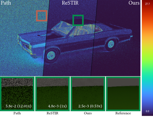 Histogram Stratification for Spatio-Temporal Reservoir SamplingIn Proceedings of the Special Interest Group on Computer Graphics and Interactive Techniques Conference Conference Papers, , 2025

2024
-
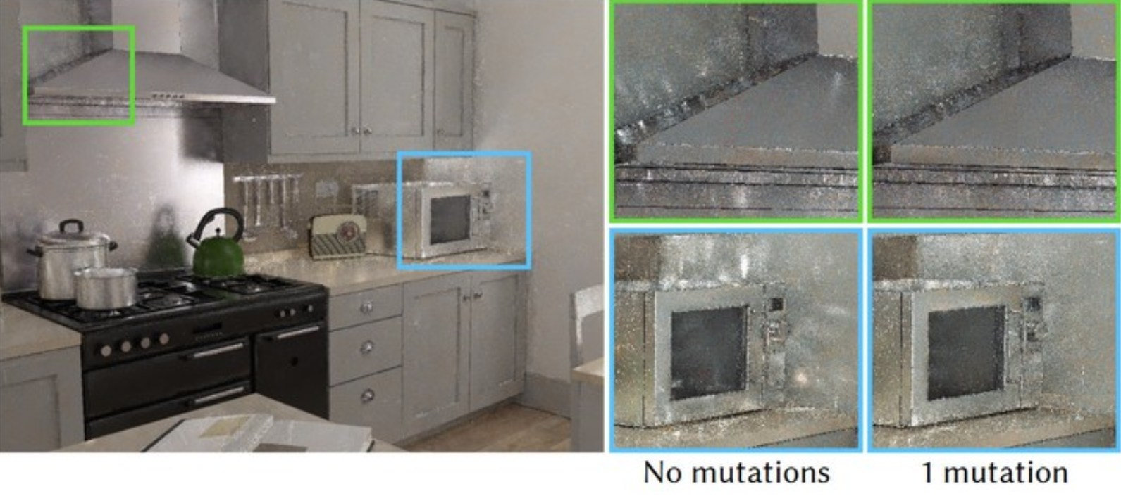 Decorrelating ReSTIR Samplers via MCMC MutationsACM Transactions on Graphics (ToG), Jan 2024
 -
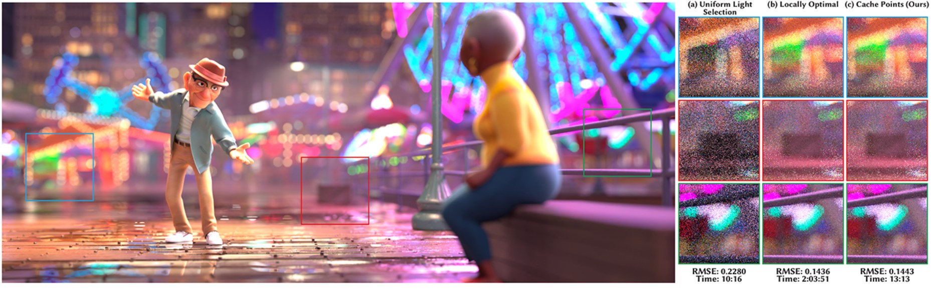 Cache Points For Production-Scale Occlusion-Aware Many-Lights Sampling And VolumetricIn DigiPro ’24: Proceedings of the Digital Production Symposium 2024, Jul 2024
 -
 A Resampled Tree for Many Lights RenderingIn ACM SIGGRAPH 2024 Talks, Denver, CO, USA, Jul 2024
 -
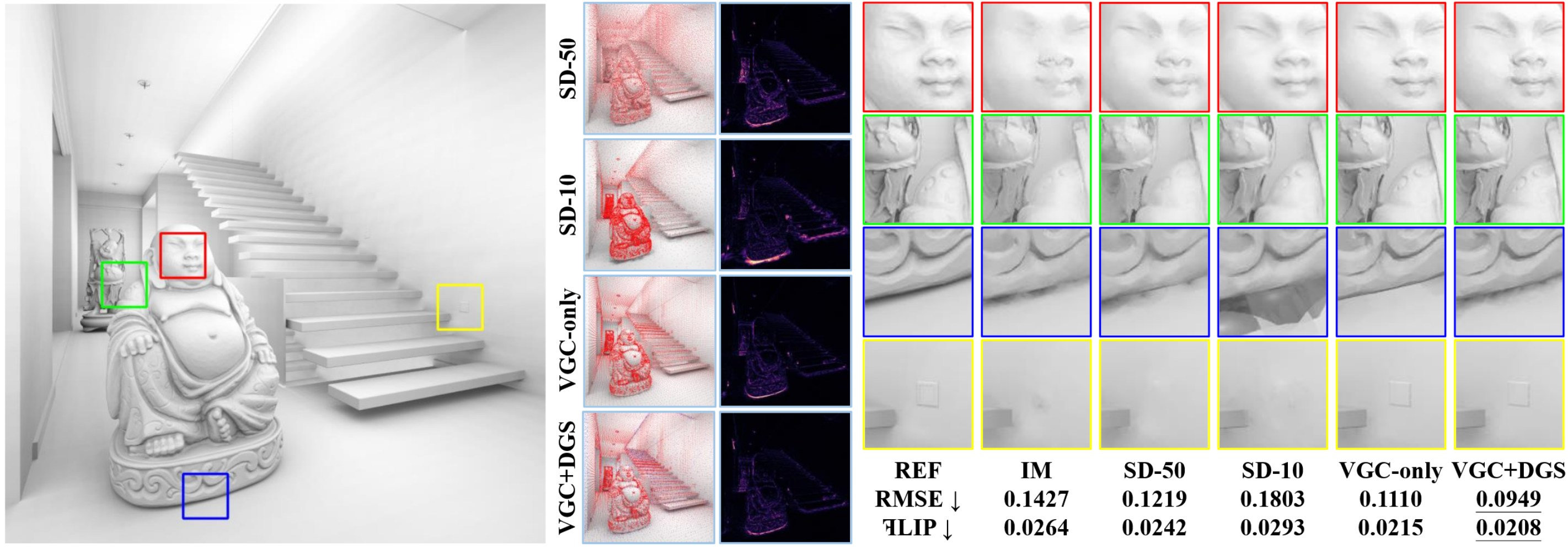


2023
-
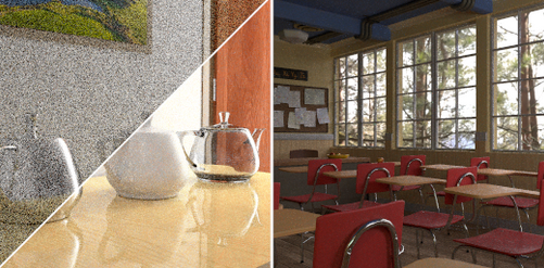 A Gentle Introduction to ReSTIR: Path Reuse in Real-timeIn ACM SIGGRAPH 2023 Courses, Los Angeles, California, Aug 2023

2022
-
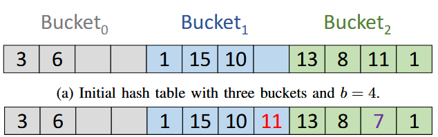 Better GPU Hash TablesAug 2022
 -
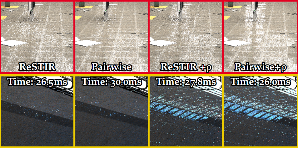 Correlations and Reuse for Fast and Accurate Physically Based Light TransportAug 2022
 -
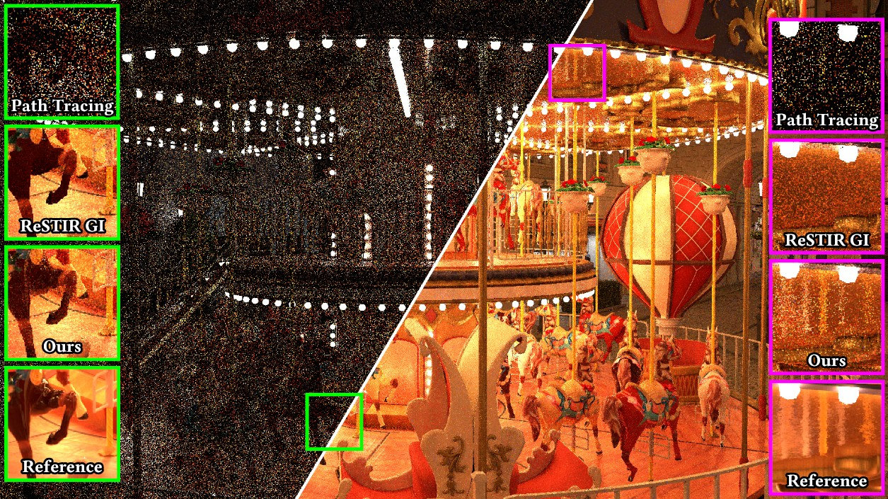


2021
-
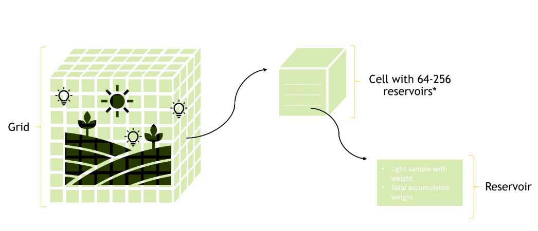
-
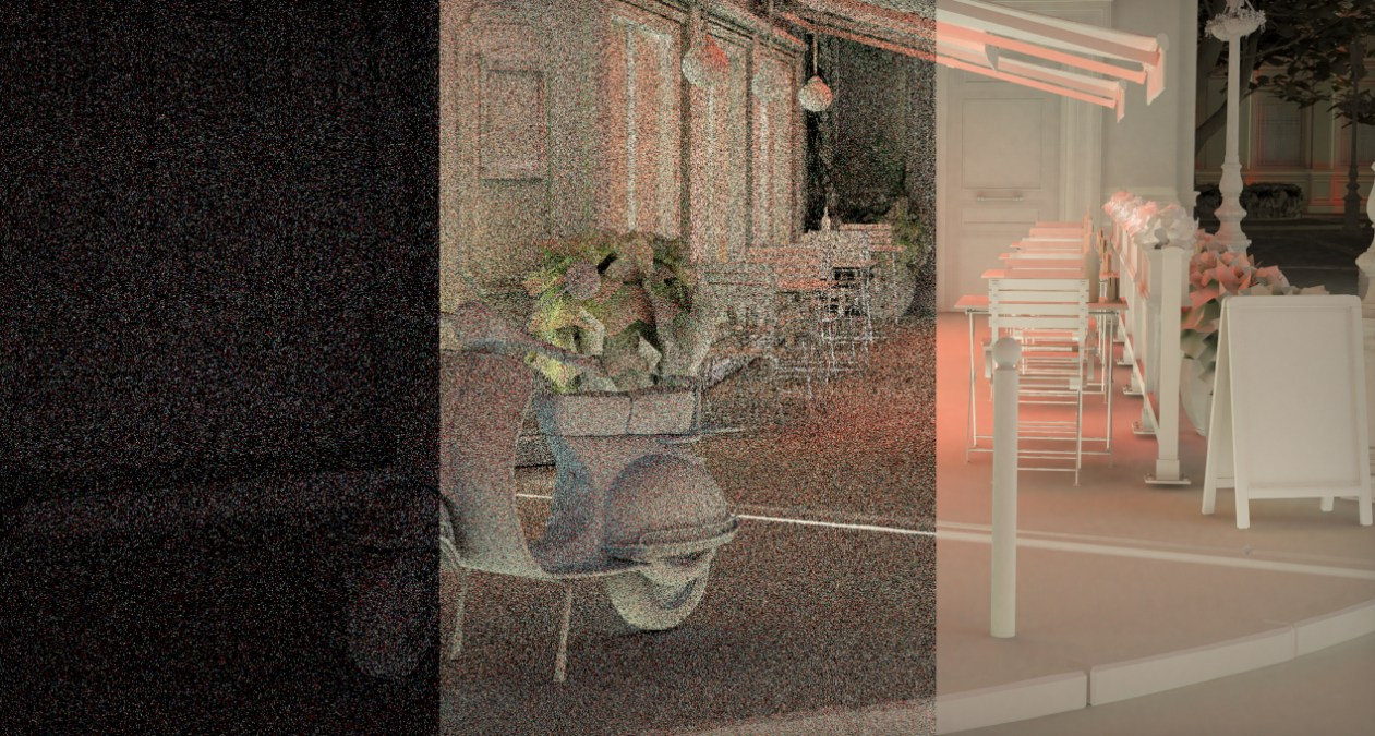 WORLD-SPACE SPATIOTEMPORAL RESERVOIR REUSE FOR RAY-TRACED GLOBAL ILLUMINATIONIn SIGGRAPH Asia 2021 Technical Communications, Tokyo, Japan, Jul 2021
 -
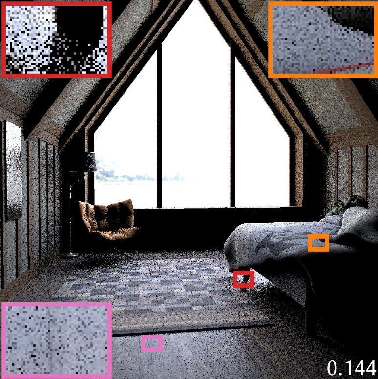


2020
-
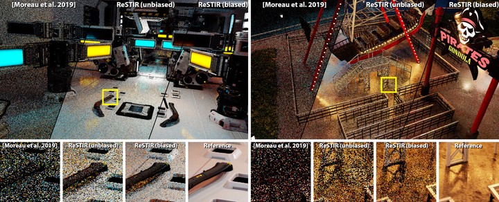 Spatiotemporal Reservoir Resampling for Real-time Ray Tracing with Dynamic Direct LightingACM Transactions on Graphics (SIGGRAPH), Jul 2020
 -
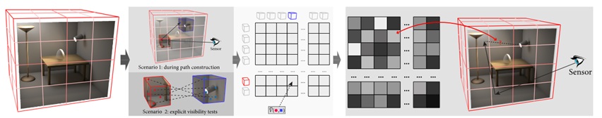 Next Event Estimation++: Visibility Mapping for Efficient Light Transport SimulationComputer Graphics Forum (Proc. of Pacific Graphics PG), Nov 2020
 -
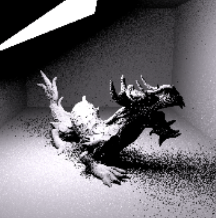 Practical Product Sampling by Fitting and Composing WarpsComputer Graphics Forum, Jul 2020


2019
-
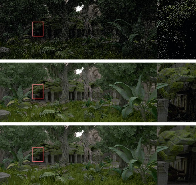 Massively Parallel Path Space FilteringCoRR, Jul 2019
 - SIGGRAPH 2019: Real-Time Ray Tracing - Special Topics and Latest Resarch- Ray-Traced Global Illumination for Games: Massively Parallel Path Space FilteringJul 2019
-
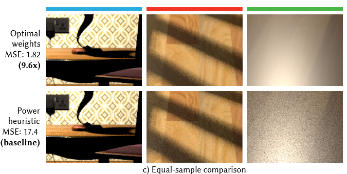


2018
-
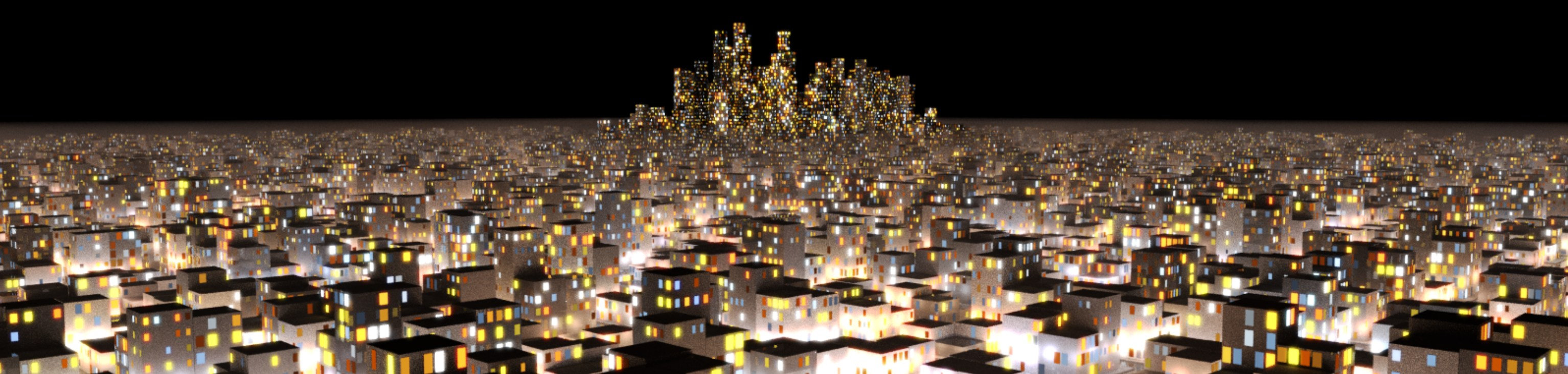 Importance Sampling of Many Lights with Adaptive Tree SplittingProc. ACM Comput. Graph. Interact. Tech., Aug 2018
 -
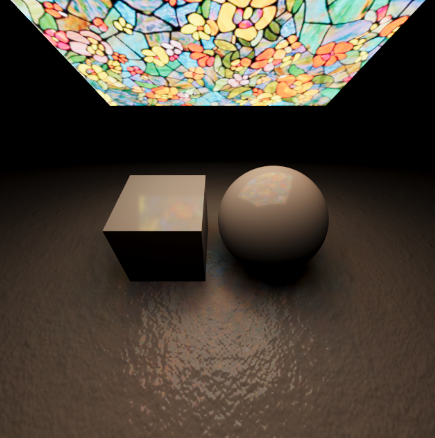 Combining analytic direct illumination and stochastic shadowsIn Proceedings of the ACM SIGGRAPH Symposium on Interactive 3D Graphics and Games, Montreal, Quebec, Canada, Aug 2018


2016

2005
-
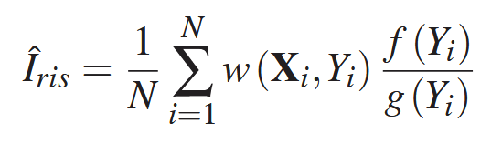 Importance Resampling for Global IlluminationIn , Jan 2005
