Adaptive Sampling in a Path Tracer
Per-Pixel Adaptive Sampling for offline Path Tracing
Adaptive sampling is a technique that allows focusing the samples on pixels that need more of them. This is useful because not all parts of a scene are equally complex to render.
Consider this modified cornell box for example:
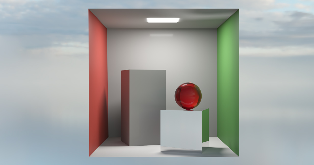
Half of the rays of this scene don’t even intersect any geometry and directly end up in the environment where the color of the environment map is computed. The variance of the radiance of these rays is very low since a given camera ray direction basically always results in the same radiance (almost) being returned.
However, the same cannot be said for the reflective caustic (the emissive light panel reflecting off the mirror small box) at the top right of the Cornell box. A camera ray that hits this region of the ceiling then has a fairly low chance of bouncing in direction of the small box to then bounce directly in the direction of the light. This makes the variance of these rays very high which really slows down the convergence of this part of the scene. As a result, we would like to shoot more rays at these pixels than at other parts of the scene to help with the convergence.
Adaptive sampling allows us to do just that. The idea is to estimate the error of each pixel of the image, compare this estimated error with a user-defined threshold \(T\) and only continue to sample the pixel if the pixel’s error is still larger than the threshold.
A very simple error metric is that of the variance of the luminance \(\sigma^2\) of the pixel. In practice, we want to estimate the variance of a pixel across the \(N\) samples \(x_k\) it has received so far.
The variance of \(N\) samples is usually computed as:
\[\sigma^2 = \frac{1}{N}\sum_{k=1}^N (x_k - \mu) ^2\]However, this approach would imply keeping the average of each pixel’s samples (which is the framebuffer itself so that’s fine) as well as the values of all samples seen so far (that’s not fine). Every time we want to estimate the error of a single pixel, we would then have to loop over all the previous samples to compute their difference with the average and get our variance \(\sigma^2\). Keeping track of all the samples is infeasible in terms of memory consumption (that would be 2GB of RAM/VRAM for a mere 256 samples’ floating-point luminance at 1080p) and looping over all the samples seen so far is computationally way too demanding.
The practical solution is to evaluate the running-variance of the \(N\) pixel samples \(x_k\):
\[\sigma^2 = \frac{1}{N - 1} \left(\sum_{k=1}^N x_k^2 - \left( \sum_{k=1}^N x_k \right)^2\right)\]Note
Due to the nature of floating point numbers, this formula can have some precision issues. This Wikipedia article presents good alternatives.
With the variance, we can compute a 95% confidence interval \(I\):
\[I = 1.96 \frac{\sigma}{\sqrt{N}}\]This 95% confidence interval gives us a range around our samples mean \(\mu\) and we can be 95% sure that, for the current number of samples \(N\) and and their variance \(\sigma\) that we used to compute this interval, the converged mean (true mean) of an infinite amount of samples is in that interval.
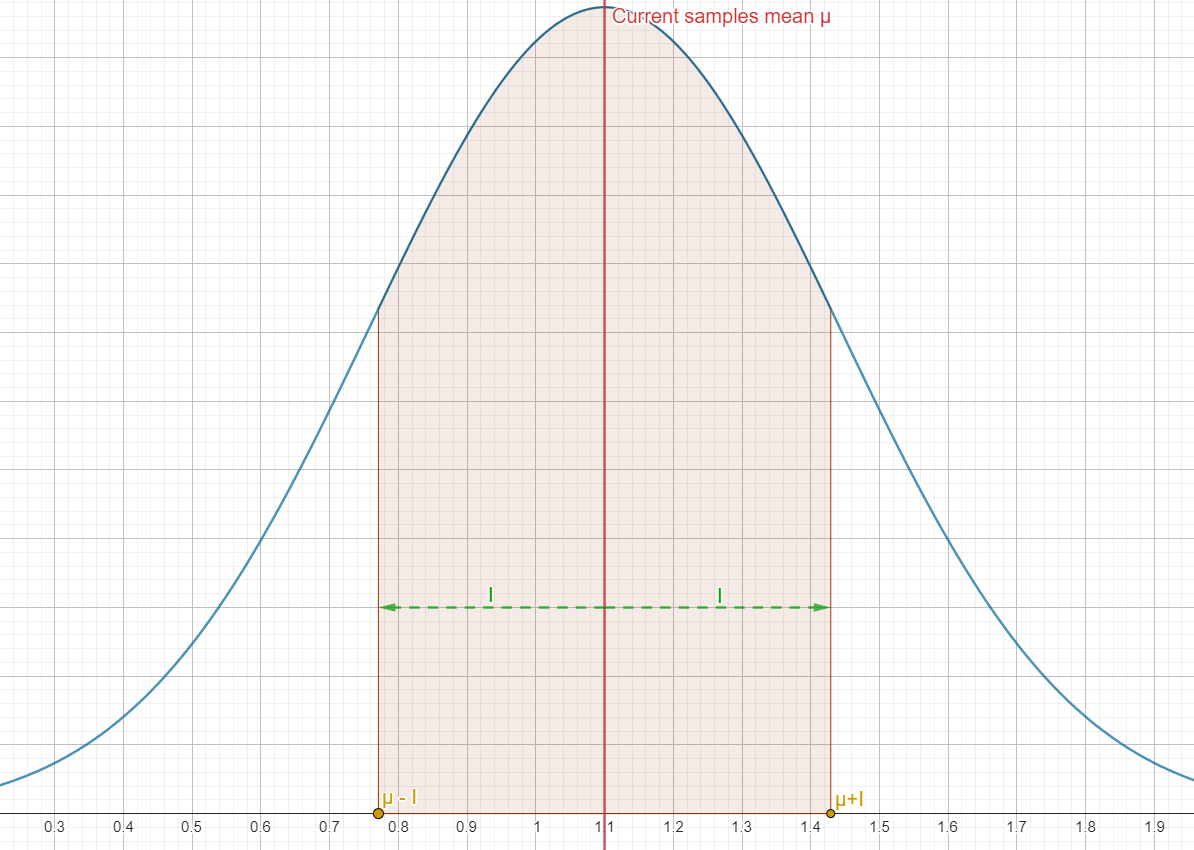
Judging by how \(I\) is computed, it is easy to see that as the number of samples \(N\) increases or the variance \(\sigma^2\) decreases (and thus \(\sigma\) decreases too), \(I\) decreases.
That should make sense since as we increase the number of samples, our mean \(\mu\) should get closer and closer to the “true” mean value of the pixel (which is the value of the fully converged pixel when an infinite amount of samples are averaged together).
If \(I\) gets smaller, this means for our \(\mu\) that it also gets closer to the “true” mean and that is the sign that our pixel has converged a little more.
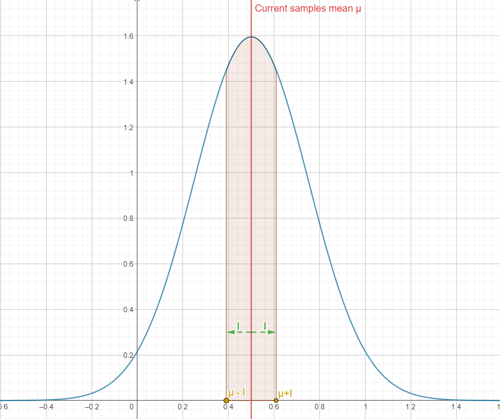
Knowing that we can interpret \(I\) as a measure of the convergence of our pixel, the question now becomes:
When do we assume that our pixel has sufficiently converged and stop sampling?
We use that user-given threshold \(T\) we talked about earlier! Specifically, we can assume that if \(I \leq T\mu\), rhen that pixel has converged enough for that threshold \(T\). As a practical example, consider \(T=0\). We then have:
\[\displaylines{I \leq T\mu \\ I \leq 0}\]If \(I=0\), then the interval completely collapses on \(\mu\). Said otherwise, \(\mu\) is the true mean and our pixel has completely converged. Thus, for \(T=0\), we will only stop sampling the pixel when it has fully converged.
In practice, having \(I=0\) is infeasible. After some experimentations a \(T\) threshold of \(0.1\) seems to target a visually very reasonable amount of noise. Any \(T\) lower than that represents quite the overhead in terms of rendering times but can still provide some improvements on the perceived level of noise:
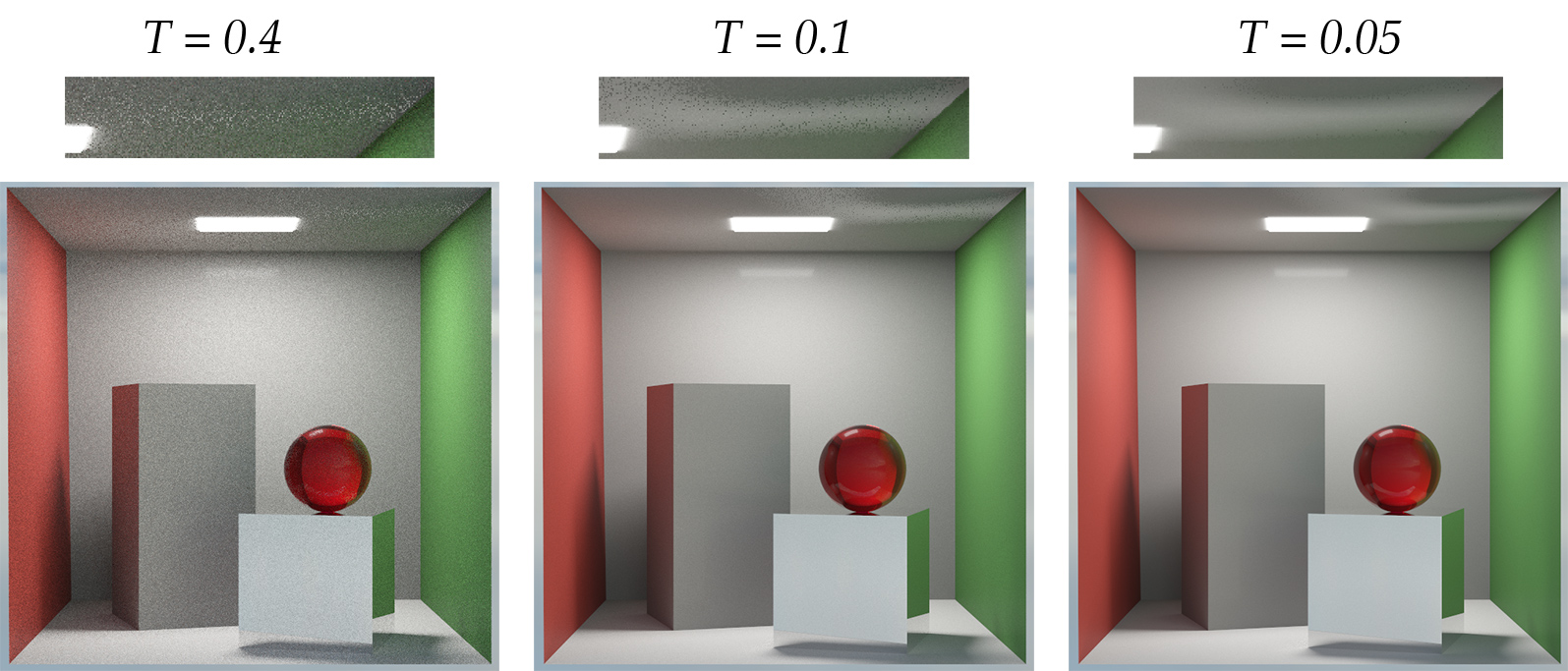
Now if you look at the render with \(T=0.1\), you’ll notice that the caustic on the ceiling is awkwardly noisier than the rest of the image. There are some “holes” in the caustic (easy to see when you compare it to the \(T=0.05\) render).
This is an issue of the per-pixel approach used here: because that caustic has so much variance, it is actually possible that we sample a pixel on the ceiling 50 times (arbitrary number) without ever finding a path to the light. The sampled pixel will then remain gray-ish (diffuse color of the ceiling) instead of being bright because of the caustic. Our evaluation of the error of this pixel will then assume that it has converged since it has gone through 50 samples without that much of a change in radiance, meaning that it has a low variance, meaning that we can stop sampling it.
But we shouldn’t! If we had sampled it maybe 50 more times, we would have probably found a path that leads to the light, spiking the variance of the pixel which in turn would be sampled until the variance has attenuated enough so that our confidence interval \(I\) is small again and gets below our threshold.
One solution is simply to increase the minimum number of samples that must be traced through a pixel before evaluating its error. This way, the pixels of the image all get a chance to show their true variance and can’t escape the adaptive sampling strategy!
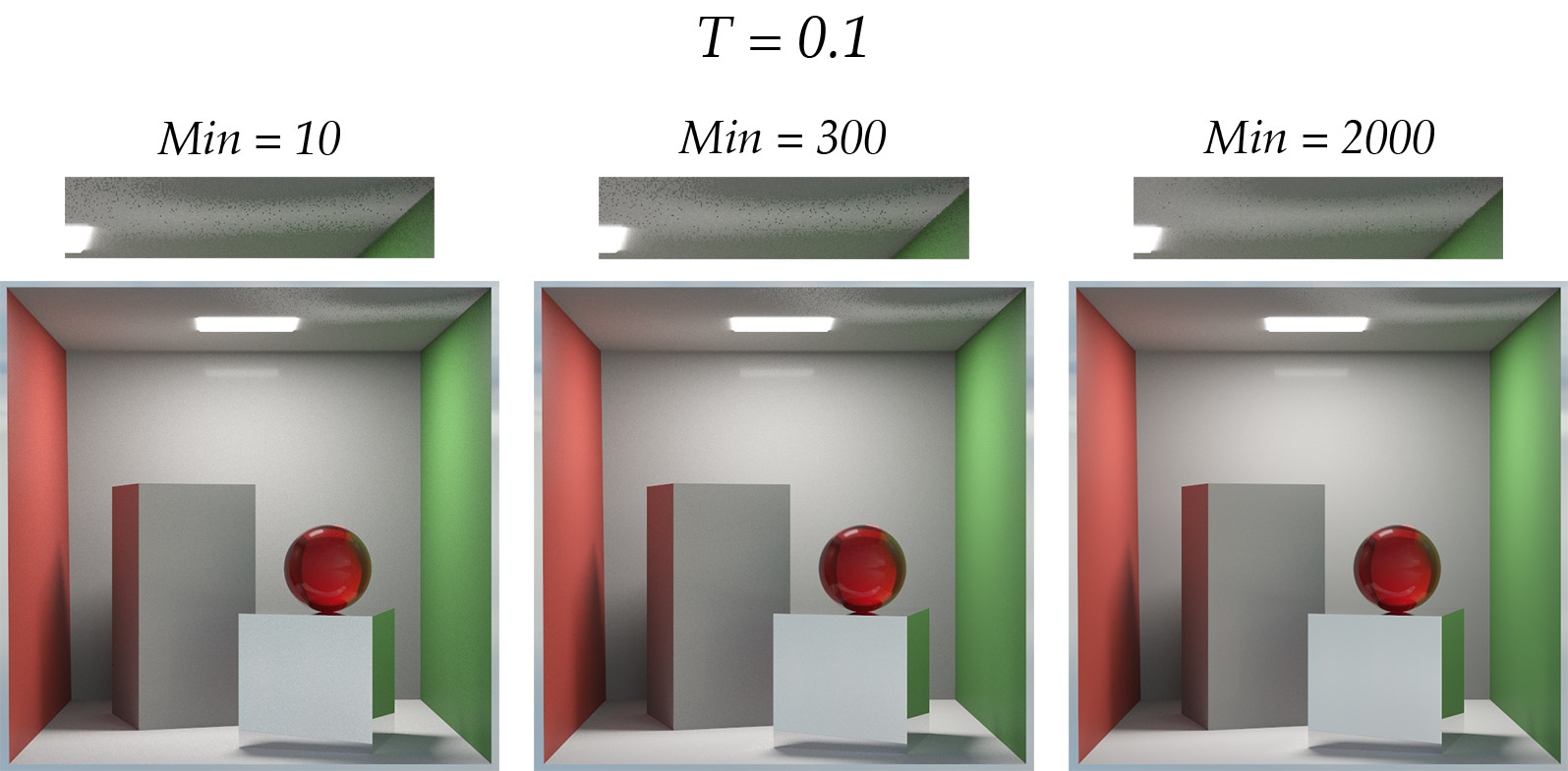
This is however a poor solution since this forces all pixels of the image to be sampled at least 100 times, even the ones that would only need 50 samples. This is a waste of computational resources.
A better way of estimating the error of the scene will be presented in a future blog post on “Hierarchical Adaptive Sampling”.
Nonetheless, this naive way of estimating the error of a pixel can provide very appreciable speedups in rendering time.
| $T = 0.1$ | 90% | 95% | 99% |
|---|---|---|---|
| Bistro | 3626/1601 (2.26x) | 5104/1782 (2.86x) | 12068/2057 (5.8x) |
| McLaren P1 | 178/74 (2.4x) | 492/198 (2.48x) | 3227/480 (6.7x) |
| The White Room 4 bounces | 98/54 (1.8x) | 130/58 (2.24x) | 270/78 (3.46x) |
| The White Room 16 bounces | 1020/347 (2.9x) | 1668/656 (2.54x) | 2629/459 (5.7x) |
| $T=0.3$ | 90% | 95% | 99% |
| Bistro | 384/152 (2.53x) | 551/170 (3.24x) | 1124/196 (5.73x) |
| McLaren P1 | 17/10 (1.7x) | 43/19 (2.26x) | 244/50 (4.88x) |
| The White Room 4 bounces | 10/6 (1.67x) | 15/7 (2.14x) | 31/8 (3.88x) |
| The White Room 16 bounces | 69/26 (2.65x) | 111/31 (3.58x) | 268/39 (6.87x) |
A few notes:
- Times are in second
- All renders with adaptive sampling were rendered with 96 minimum samples.
-
Do not compare times between categories (categories are 90%/95%/99% and \(T=0.1\) or \(T=0.3\)). Some images were rendered with the GPU limiter feature of my renderer (to avoid burning my GPU for hours) and so times are not always comparable between categories. Two images of the same category (and of the same scene, i.e. do not compare times of the Bistro with times of the Mc Laren P1) were rendered with the exact same settings so times are comparable there.
-
You may have noticed that the images with that used the adaptive sampling are noisier than the images rendered without (most noticeable with \(T=0.3\)). This is because without the adaptive sampling, the renderer had no choice but to render every pixels of the image until 90/95/99% have reached the threshold (\(T=0.1\) or \(T=0.3\)). This is a massive waste of time, especially if you intend to use a denoiser as the final step of the rendering process. As a matter of fact, Open Image Denoise (which is the denoiser in my renderer used at the time of writing this post) with normals and albedo AOVs behaves very well on an image rendered with a \(T=0.3\) threshold and adaptive sampling on. There’s almost no reason not to use adaptive sampling when denoising the render (except maybe for the “holes” issue explained below).
- The holes are still there! Even at \(T=0.1\), on the Mc Laren, below the right mirror :( Unfortunately yes. The only proper solution that I can imagine is to either increase the minimum number of samples before kicking off the adaptive sampling or use a hierarchical solution
, which I haven’t explored in practice yet.